PaddleX 3.0 公式识别(formula_recognition)模型产线实践教程
PaddleX 提供了丰富的模型产线,模型产线由一个或多个模型组合实现,每个模型产线都能够解决特定的场景任务问题。PaddleX 所提供的模型产线均支持快速体验,如果效果不及预期,也同样支持使用私有数据微调模型,并且 PaddleX 提供了 Python API,方便将产线集成到个人项目中。在使用之前,您首先需要安装 PaddleX, 安装方式请参考 PaddleX本地安装教程。请注意,本文档是公式识别产线的实践教程,提供一些实践经验,并非该产线的完整使用教程,完整的使用教程请参考 PaddleX 公式识别产线。
1. 选择模型产线
公式作为科学文献、技术文档及教育资料的核心知识载体,承载着人类文明的抽象逻辑与数学表达。公式识别旨在对学术论文、工程图纸等场景中的行间公式、行内公式及手写公式进行解析,将其转化为结构化的LaTeX代码。在科研领域的问题求解、定理推导、知识库构建等方面具有广泛的应用。同时,公式识别在科研数据集构建中发挥着重要的作用。通过与版面区域检测、文本检测、文本识别、顺序预测等OCR类模型结合,我们可以将图像中的公式代码、文本内容等零散、没有语义的结构化数据,转化为具有语义上下文的markdown代码,构建大模型数据的QA对,从而提升大模型对于科研论文的理解和感知能力。
首先,需要根据任务场景,选择对应的 PaddleX 产线,本节以公式识别产线的结果后处理优化为例,希望获取科研论文图像中的丰富的语料信息,对应 PaddleX 的公式识别模块、版面区域检测模块、文档图像方向分类模块和文本图像矫正模块,可以在公式识别产线中使用。如果无法确定任务和产线的对应关系,您可以在 PaddleX 支持的模型产线列表中了解相关产线的能力介绍。
2. 模型列表
公式识别产线中包含必选的公式识别模块,以及可选的版面区域检测模块、文档图像方向分类模块和文本图像矫正模块。其中,文档图像方向分类模块和文本图像矫正模块作为文档预处理子产线被集成到公式识别产线中。每个模块都包含多个模型,您可以根据下方的基准测试数据选择使用的模型。
如果您更注重模型的精度,请选择精度较高的模型;如果您更在意模型的推理速度,请选择推理速度较快的模型;如果您关注模型的存储大小,请选择存储体积较小的模型。
文档图像方向分类模块(可选):
| 模型 | 模型下载链接 | Top-1 Acc(%) | GPU推理耗时(ms) [常规模式 / 高性能模式] |
CPU推理耗时(ms) [常规模式 / 高性能模式] |
模型存储大小(MB) | 介绍 |
|---|---|---|---|---|---|---|
| PP-LCNet_x1_0_doc_ori | 推理模型/训练模型 | 99.06 | 2.62 / 0.59 | 3.24 / 1.19 | 7 | 基于PP-LCNet_x1_0的文档图像分类模型,含有四个类别,即0度,90度,180度,270度 |
文本图像矫正模块(可选):
| 模型 | 模型下载链接 | CER | GPU推理耗时(ms) [常规模式 / 高性能模式] |
CPU推理耗时(ms) [常规模式 / 高性能模式] |
模型存储大小(MB) | 介绍 |
|---|---|---|---|---|---|---|
| UVDoc | 推理模型/训练模型 | 0.179 | 19.05 / 19.05 | - / 869.82 | 30.3 | 高精度文本图像矫正模型 |
版面区域检测模块(可选):
| 模型 | 模型下载链接 | mAP(0.5)(%) | GPU推理耗时(ms) [常规模式 / 高性能模式] |
CPU推理耗时(ms) [常规模式 / 高性能模式] |
模型存储大小(MB) | 介绍 |
|---|---|---|---|---|---|---|
| PP-DocLayout-L | 推理模型/训练模型 | 90.4 | 33.59 / 33.59 | 503.01 / 251.08 | 123.76 | 基于RT-DETR-L在包含中英文论文、杂志、合同、书本、试卷和研报等场景的自建数据集训练的高精度版面区域定位模型 |
| PP-DocLayout-M | 推理模型/训练模型 | 75.2 | 13.03 / 4.72 | 43.39 / 24.44 | 22.578 | 基于PicoDet-L在包含中英文论文、杂志、合同、书本、试卷和研报等场景的自建数据集训练的精度效率平衡的版面区域定位模型 |
| PP-DocLayout-S | 推理模型/训练模型 | 70.9 | 11.54 / 3.86 | 18.53 / 6.29 | 4.834 | 基于PicoDet-S在中英文论文、杂志、合同、书本、试卷和研报等场景上自建数据集训练的高效率版面区域定位模型 |
❗ 以上列出的是版面区域检测模块重点支持的3个核心模型,该模块总共支持6个全量模型,包含多个预定义了不同类别的模型,完整的模型列表如下:
👉模型列表详情
* 17类版面区域检测模型,包含17个版面常见类别,分别是:段落标题、图片、文本、数字、摘要、内容、图表标题、公式、表格、表格标题、参考文献、文档标题、脚注、页眉、算法、页脚、印章| 模型 | 模型下载链接 | mAP(0.5)(%) | GPU推理耗时(ms) [常规模式 / 高性能模式] |
CPU推理耗时(ms) [常规模式 / 高性能模式] |
模型存储大小(MB) | 介绍 |
|---|---|---|---|---|---|---|
| PicoDet-S_layout_17cls | 推理模型/训练模型 | 87.4 | 8.80 / 3.62 | 17.51 / 6.35 | 4.8 | 基于PicoDet-S轻量模型在中英文论文、杂志和研报等场景上自建数据集训练的高效率版面区域定位模型 |
| PicoDet-L_layout_17cls | 推理模型/训练模型 | 89.0 | 12.60 / 10.27 | 43.70 / 24.42 | 22.6 | 基于PicoDet-L在中英文论文、杂志和研报等场景上自建数据集训练的效率精度均衡版面区域定位模型 |
| RT-DETR-H_layout_17cls | 推理模型/训练模型 | 98.3 | 115.29 / 101.18 | 964.75 / 964.75 | 470.2 | 基于RT-DETR-H在中英文论文、杂志和研报等场景上自建数据集训练的高精度版面区域定位模型 |
| 模型 | 模型下载链接 | mAP(0.5)(%) | GPU推理耗时(ms) [常规模式 / 高性能模式] |
CPU推理耗时(ms) [常规模式 / 高性能模式] |
模型存储大小(MB) | 介绍 |
|---|---|---|---|---|---|---|
| PP-DocLayout-L | 推理模型/训练模型 | 90.4 | 33.59 / 33.59 | 503.01 / 251.08 | 123.76 | 基于RT-DETR-L在包含中英文论文、杂志、合同、书本、试卷和研报等场景的自建数据集训练的高精度版面区域定位模型 |
| PP-DocLayout-M | 推理模型/训练模型 | 75.2 | 13.03 / 4.72 | 43.39 / 24.44 | 22.578 | 基于PicoDet-L在包含中英文论文、杂志、合同、书本、试卷和研报等场景的自建数据集训练的精度效率平衡的版面区域定位模型 |
| PP-DocLayout-S | 推理模型/训练模型 | 70.9 | 11.54 / 3.86 | 18.53 / 6.29 | 4.834 | 基于PicoDet-S在中英文论文、杂志、合同、书本、试卷和研报等场景上自建数据集训练的高效率版面区域定位模型 |
公式识别模块:
| 模型 | 模型下载链接 | Avg-BLEU(%) | GPU推理耗时(ms) [常规模式 / 高性能模式] |
CPU推理耗时(ms) [常规模式 / 高性能模式] |
模型存储大小(MB) | 介绍 |
|---|---|---|---|---|---|---|
| UniMERNet | 推理模型/训练模型 | 86.13 | 1311.84 / 1311.84 | - / 8288.07 | 1530 | UniMERNet是由上海AI Lab研发的一款公式识别模型。该模型采用Donut Swin作为编码器,MBartDecoder作为解码器,并通过在包含简单公式、复杂公式、扫描捕捉公式和手写公式在内的一百万数据集上进行训练,大幅提升了模型对真实场景公式的识别准确率 |
| PP-FormulaNet-S | 推理模型/训练模型 | 87.12 | 182.25 / 182.25 | - / 254.39 | 167.9 | PP-FormulaNet 是由百度飞桨视觉团队开发的一款先进的公式识别模型,支持5万个常见LateX源码词汇的识别。PP-FormulaNet-S 版本采用了 PP-HGNetV2-B4 作为其骨干网络,通过并行掩码和模型蒸馏等技术,大幅提升了模型的推理速度,同时保持了较高的识别精度,适用于简单印刷公式、跨行简单印刷公式等场景。而 PP-FormulaNet-L 版本则基于 Vary_VIT_B 作为骨干网络,并在大规模公式数据集上进行了深入训练,在复杂公式的识别方面,相较于PP-FormulaNet-S表现出显著的提升,适用于简单印刷公式、复杂印刷公式、手写公式等场景。 |
| PP-FormulaNet-L | 推理模型/训练模型 | 92.13 | 1482.03 / 1482.03 | - / 3131.54 | 695 | |
| LaTeX_OCR_rec | 推理模型/训练模型 | 71.63 | 1088.89 / 1088.89 | - / - | 99 | LaTeX-OCR是一种基于自回归大模型的公式识别算法,通过采用 Hybrid ViT 作为骨干网络,transformer作为解码器,显著提升了公式识别的准确性。 |
测试环境说明:
- 性能测试环境
- 测试数据集:
- 文档图像方向分类模型:PaddleX自建的数据集,覆盖证件和文档等多个场景,包含 1000 张图片。
- 文本图像矫正模型:DocUNet。
- 版面区域检测模型:PaddleOCR 自建的版面区域检测数据集,包含中英文论文、杂志、合同、书本、试卷和研报等常见的 500 张文档类型图片。
- 17类区域检测模型:PaddleOCR 自建的版面区域检测数据集,包含中英文论文、杂志和研报等常见的 892 张文档类型图片。
- 公式识别模型:PaddleX 内部自建公式识别测试集。
- 硬件配置:
- GPU:NVIDIA Tesla T4
- CPU:Intel Xeon Gold 6271C @ 2.60GHz
- 软件环境:
- Ubuntu 20.04 / CUDA 11.8 / cuDNN 8.9 / TensorRT 8.6.1.6
- paddlepaddle 3.0.0 / paddlex 3.0.3
- 测试数据集:
- 推理模式说明
| 模式 | GPU配置 | CPU配置 | 加速技术组合 |
|---|---|---|---|
| 常规模式 | FP32精度 / 无TRT加速 | FP32精度 / 8线程 | PaddleInference |
| 高性能模式 | 选择先验精度类型和加速策略的最优组合 | FP32精度 / 8线程 | 选择先验最优后端(Paddle/OpenVINO/TRT等) |
3. 快速体验
PaddleX 提供了两种本地体验的方式,你可以在本地使用命令行或 Python 体验公式识别的效果。在本地使用公式识别产线前,请确保您已经按照PaddleX本地安装教程完成了PaddleX的wheel包安装。
首先获取产线默认配置文件,由于公式识别任务属于公式识别产线,因此执行以下命令即可获取默认配置文件:
获取的保存在./my_path/formula_recognition.yaml,修改配置文件,即可对产线各项配置进行自定义。
pipeline_name: formula_recognition

use_layout_detection: True
use_doc_preprocessor: True

SubModules:
  LayoutDetection:
    module_name: layout_detection
    model_name: PP-DocLayout-L
    model_dir: null
    threshold: 0.5
    layout_nms: True
    layout_unclip_ratio: 1.0
    layout_merge_bboxes_mode: "large"
    batch_size: 1

  FormulaRecognition:
    module_name: formula_recognition
    model_name: PP-FormulaNet-L
    model_dir: null
    batch_size: 5

SubPipelines:
  DocPreprocessor:
    pipeline_name: doc_preprocessor
    use_doc_orientation_classify: True
    use_doc_unwarping: True
    SubModules:
      DocOrientationClassify:
        module_name: doc_text_orientation
        model_name: PP-LCNet_x1_0_doc_ori
        model_dir: null
        batch_size: 1
      DocUnwarping:
        module_name: image_unwarping
        model_name: UVDoc
        model_dir: null
        batch_size: 1
随后,加载自定义配置文件 ./my_path/formula_recognition.yaml,参考以下本地体验中的命令行方式或 Python 脚本方式进行在线体验。
3.1 本地体验 ———— 命令行方式
运行以下代码前,请您下载示例图片到本地。自定义配置文件保存在 ./my_path/formula_recognition.yaml ,则只需执行:
paddlex --pipeline ./my_path/formula_recognition.yaml \
        --input general_formula_recognition_001.png \
        --save_path ./output/ \
        --device gpu:0
👉 运行后,得到的结果为:(点击展开)
{'res': {'input_path': 'general_formula_recognition_001.png', 'page_index': None, 'model_settings': {'use_doc_preprocessor': True, 'use_layout_detection': True}, 'doc_preprocessor_res': {'input_path': None, 'page_index': None, 'model_settings': {'use_doc_orientation_classify': True, 'use_doc_unwarping': True}, 'angle': 0}, 'layout_det_res': {'input_path': None, 'page_index': None, 'boxes': [{'cls_id': 2, 'label': 'text', 'score': 0.9856467843055725, 'coordinate': [90.53296, 1086.6606, 659.29224, 1553.293]}, {'cls_id': 2, 'label': 'text', 'score': 0.9839824438095093, 'coordinate': [92.88306, 127.662445, 665.87213, 397.32486]}, {'cls_id': 2, 'label': 'text', 'score': 0.9763191342353821, 'coordinate': [698.58154, 591.1726, 1292.9592, 748.10815]}, {'cls_id': 2, 'label': 'text', 'score': 0.9720773696899414, 'coordinate': [697.6456, 752.4787, 1289.5938, 883.3215]}, {'cls_id': 2, 'label': 'text', 'score': 0.9697079658508301, 'coordinate': [704.2085, 82.100555, 1305.1221, 187.76593]}, {'cls_id': 2, 'label': 'text', 'score': 0.9693678617477417, 'coordinate': [93.96658, 799.32465, 660.9802, 901.3609]}, {'cls_id': 2, 'label': 'text', 'score': 0.9682682156562805, 'coordinate': [691.67224, 1513.8839, 1283.6678, 1639.4484]}, {'cls_id': 2, 'label': 'text', 'score': 0.9675215482711792, 'coordinate': [701.09216, 287.9879, 1300.3129, 391.5937]}, {'cls_id': 7, 'label': 'formula', 'score': 0.9653083682060242, 'coordinate': [728.5991, 441.6336, 1221.3561, 571.0758]}, {'cls_id': 2, 'label': 'text', 'score': 0.9622206687927246, 'coordinate': [697.2456, 958.34705, 1288.1101, 1033.6886]}, {'cls_id': 7, 'label': 'formula', 'score': 0.9607033729553223, 'coordinate': [155.68298, 923.9154, 599.2244, 1036.6406]}, {'cls_id': 7, 'label': 'formula', 'score': 0.9583883881568909, 'coordinate': [811.17883, 1057.8389, 1175.9386, 1118.4575]}, {'cls_id': 7, 'label': 'formula', 'score': 0.9581522941589355, 'coordinate': [778.09656, 208.75406, 1225.2172, 267.90875]}, {'cls_id': 7, 'label': 'formula', 'score': 0.9572290778160095, 'coordinate': [757.6239, 1211.8169, 1189.6959, 1267.46]}, {'cls_id': 7, 'label': 'formula', 'score': 0.9553850293159485, 'coordinate': [724.06775, 1332.8228, 1255.077, 1470.4421]}, {'cls_id': 2, 'label': 'text', 'score': 0.9528529644012451, 'coordinate': [88.130035, 1557.6594, 657.3352, 1632.5967]}, {'cls_id': 7, 'label': 'formula', 'score': 0.9524679183959961, 'coordinate': [117.79787, 714.38403, 614.4141, 773.8457]}, {'cls_id': 2, 'label': 'text', 'score': 0.9510412216186523, 'coordinate': [97.06323, 479.18585, 663.7608, 536.5512]}, {'cls_id': 7, 'label': 'formula', 'score': 0.949083149433136, 'coordinate': [165.51418, 558.26685, 598.7732, 614.4641]}, {'cls_id': 2, 'label': 'text', 'score': 0.944157600402832, 'coordinate': [97.41104, 639.0248, 662.76086, 693.0067]}, {'cls_id': 2, 'label': 'text', 'score': 0.9437134265899658, 'coordinate': [696.00916, 1139.0691, 1286.3, 1188.8279]}, {'cls_id': 7, 'label': 'formula', 'score': 0.9262938499450684, 'coordinate': [196.19836, 425.07648, 568.3433, 452.05084]}, {'cls_id': 7, 'label': 'formula', 'score': 0.9207614064216614, 'coordinate': [853.4679, 908.78235, 1131.8585, 933.9021]}, {'cls_id': 7, 'label': 'formula', 'score': 0.9098795652389526, 'coordinate': [165.65845, 129.02527, 512.86633, 155.41736]}, {'cls_id': 19, 'label': 'formula_number', 'score': 0.9049411416053772, 'coordinate': [1245.7465, 1079.0446, 1286.4237, 1105.475]}, {'cls_id': 19, 'label': 'formula_number', 'score': 0.9025103449821472, 'coordinate': [1246.6572, 1229.8922, 1286.7461, 1255.7975]}, {'cls_id': 19, 'label': 'formula_number', 'score': 0.9007143974304199, 'coordinate': [1246.525, 909.0211, 1287.5856, 935.64417]}, {'cls_id': 7, 'label': 'formula', 'score': 0.8995094895362854, 'coordinate': [96.4274, 234.94318, 295.6733, 265.9768]}, {'cls_id': 19, 'label': 'formula_number', 'score': 0.8980057239532471, 'coordinate': [1252.8303, 493.0625, 1294.4944, 519.0]}, {'cls_id': 2, 'label': 'text', 'score': 0.8979238271713257, 'coordinate': [725.74915, 396.12943, 1262.9354, 422.97177]}, {'cls_id': 19, 'label': 'formula_number', 'score': 0.8966280221939087, 'coordinate': [1242.1687, 1473.5837, 1283.3108, 1499.4875]}, {'cls_id': 2, 'label': 'text', 'score': 0.8917680382728577, 'coordinate': [94.72511, 1058.2068, 442.26758, 1081.7258]}, {'cls_id': 2, 'label': 'text', 'score': 0.8913338780403137, 'coordinate': [697.516, 1286.2783, 1083.2262, 1310.8098]}, {'cls_id': 19, 'label': 'formula_number', 'score': 0.8882836699485779, 'coordinate': [1270.5066, 221.21191, 1299.9436, 247.35437]}, {'cls_id': 7, 'label': 'formula', 'score': 0.8880225419998169, 'coordinate': [96.42808, 1320.5374, 263.84195, 1346.2654]}, {'cls_id': 19, 'label': 'formula_number', 'score': 0.8837041258811951, 'coordinate': [634.8523, 428.02948, 662.4497, 453.44977]}, {'cls_id': 19, 'label': 'formula_number', 'score': 0.8757179379463196, 'coordinate': [631.19507, 939.25635, 658.7859, 965.2036]}, {'cls_id': 19, 'label': 'formula_number', 'score': 0.8704060316085815, 'coordinate': [635.2284, 576.11304, 661.34033, 602.0388]}, {'cls_id': 19, 'label': 'formula_number', 'score': 0.8691984415054321, 'coordinate': [631.19885, 1001.11475, 658.0812, 1026.0303]}, {'cls_id': 19, 'label': 'formula_number', 'score': 0.8690404891967773, 'coordinate': [633.90576, 730.33673, 660.7864, 755.97186]}, {'cls_id': 7, 'label': 'formula', 'score': 0.850570023059845, 'coordinate': [1091.3225, 1598.8713, 1277.7903, 1622.5471]}, {'cls_id': 7, 'label': 'formula', 'score': 0.8437846302986145, 'coordinate': [694.82336, 1611.6716, 861.55835, 1635.6594]}, {'cls_id': 7, 'label': 'formula', 'score': 0.7667798399925232, 'coordinate': [918.3441, 1618.5991, 1010.3434, 1640.8501]}, {'cls_id': 3, 'label': 'number', 'score': 0.76311856508255, 'coordinate': [1297.2578, 8.878933, 1310.373, 28.363262]}, {'cls_id': 7, 'label': 'formula', 'score': 0.7419516444206238, 'coordinate': [382.79633, 267.88034, 515.84784, 296.95737]}, {'cls_id': 7, 'label': 'formula', 'score': 0.7332333922386169, 'coordinate': [100.81209, 508.70236, 253.98692, 535.70435]}, {'cls_id': 7, 'label': 'formula', 'score': 0.7307442426681519, 'coordinate': [1116.9696, 1573.1519, 1193.5485, 1595.2427]}, {'cls_id': 7, 'label': 'formula', 'score': 0.7140133380889893, 'coordinate': [539.10486, 480.36127, 662.8451, 508.7262]}, {'cls_id': 7, 'label': 'formula', 'score': 0.6723657846450806, 'coordinate': [245.42169, 160.63435, 308.15094, 185.54918]}, {'cls_id': 7, 'label': 'formula', 'score': 0.6489072442054749, 'coordinate': [175.75285, 350.04596, 243.64375, 376.14642]}, {'cls_id': 7, 'label': 'formula', 'score': 0.6118927001953125, 'coordinate': [849.2805, 619.52155, 960.4343, 646.4367]}, {'cls_id': 7, 'label': 'formula', 'score': 0.6036254167556763, 'coordinate': [256.20428, 323.1073, 327.27972, 349.5608]}, {'cls_id': 7, 'label': 'formula', 'score': 0.6015271544456482, 'coordinate': [696.23254, 1561.4348, 900.39685, 1586.3093]}, {'cls_id': 7, 'label': 'formula', 'score': 0.5478202104568481, 'coordinate': [1262.7578, 315.4475, 1297.2837, 339.2895]}, {'cls_id': 7, 'label': 'formula', 'score': 0.5441924333572388, 'coordinate': [788.66956, 349.7992, 812.65125, 370.2704]}, {'cls_id': 7, 'label': 'formula', 'score': 0.5188493728637695, 'coordinate': [774.41125, 594.7079, 802.1969, 618.0421]}]}, 'formula_res_list': [{'rec_formula': '\\small\\begin{aligned}{\\psi_{0}(M)-\\psi(M,z)=}&{{}\\frac{(1-\\epsilon_{r})}{\\epsilon_{r}}\\frac{\\lambda^{2}c^{2}}{t_{\\operatorname{E}}^{2}\\operatorname{ln}(10)}\\times}\\\\ {}&{{}\\int_{0}^{z}d z^{\\prime}\\frac{d t}{d z^{\\prime}}\\left.\\frac{\\partial\\phi}{\\partial L}\\right|_{L=\\lambda M c^{2}/t_{\\operatorname{E}}},}\\\\ \\end{aligned}', 'formula_region_id': 1, 'dt_polys': ([728.5991, 441.6336, 1221.3561, 571.0758],)}, {'rec_formula': '\\begin{aligned}{\\rho_{\\mathrm{BH}}}&{{}=\\int d M\\psi(M)M}\\\\ {}&{{}=\\frac{1-\\epsilon_{r}}{\\epsilon_{r}c^{2}}\\int_{0}^{\\infty}d z\\frac{d t}{d z}\\int d\\log_{10}L\\phi(L,z)L,}\\\\ \\end{aligned}', 'formula_region_id': 2, 'dt_polys': ([155.68298, 923.9154, 599.2244, 1036.6406],)}, {'rec_formula': '\\frac{d n}{d\\sigma}d\\sigma=\\psi_{*}\\left(\\frac{\\sigma}{\\sigma_{*}}\\right)^{\\alpha}\\frac{e^{-(\\sigma/\\sigma_{*})^{\\beta}}}{\\Gamma(\\alpha/\\beta)}\\beta\\frac{d\\sigma}{\\sigma}.', 'formula_region_id': 3, 'dt_polys': ([811.17883, 1057.8389, 1175.9386, 1118.4575],)}, {'rec_formula': '\\phi(L)\\equiv\\frac{d n}{d\\log_{10}L}=\\frac{\\phi_{*}}{(L/L_{*})^{\\gamma_{1}}+(L/L_{*})^{\\gamma_{2}}}.', 'formula_region_id': 4, 'dt_polys': ([778.09656, 208.75406, 1225.2172, 267.90875],)}, {'rec_formula': '\\small\\begin{aligned}{\\psi_{0}(M)=\\int d\\sigma\\frac{p(\\operatorname{log}_{10}M|\\operatorname{log}_{10}\\sigma)}{M\\operatorname{log}(10)}\\frac{d n}{d\\sigma}(\\sigma),}\\\\ \\end{aligned}', 'formula_region_id': 5, 'dt_polys': ([757.6239, 1211.8169, 1189.6959, 1267.46],)}, {'rec_formula': '\\small\\begin{aligned}{p(\\operatorname{log}_{10}}&{{}M|\\operatorname{log}_{10}\\sigma)=\\frac{1}{\\sqrt{2\\pi}\\epsilon_{0}}}\\\\ {}&{{}\\times\\operatorname{exp}\\left[-\\frac{1}{2}\\left(\\frac{\\operatorname{log}_{10}M-a_{\\bullet}-b_{\\bullet}\\operatorname{log}_{10}\\sigma}{\\epsilon_{0}}\\right)^{2}\\right].}\\\\ \\end{aligned}', 'formula_region_id': 6, 'dt_polys': ([724.06775, 1332.8228, 1255.077, 1470.4421],)}, {'rec_formula': '\\frac{\\partial\\psi}{\\partial t}(M,t)+\\frac{(1-\\epsilon_{r})}{\\epsilon_{r}}\\frac{\\lambda^{2}c^{2}}{t_{\\mathrm{E}}^{2}\\ln(10)}\\left.\\frac{\\partial\\phi}{\\partial L}\\right|_{L=\\lambda M c^{2}/t_{\\mathrm{v}}}=0,', 'formula_region_id': 7, 'dt_polys': ([117.79787, 714.38403, 614.4141, 773.8457],)}, {'rec_formula': '\\langle\\dot{M}(M,t)\\rangle\\psi(M,t)=\\frac{(1-\\epsilon_{r})}{\\epsilon_{r}c^{2}\\operatorname{ln}(10)}\\phi(L,t)\\frac{d L}{d M}.', 'formula_region_id': 8, 'dt_polys': ([165.51418, 558.26685, 598.7732, 614.4641],)}, {'rec_formula': '\\phi(L,t)d\\log_{10}L=\\delta(M,t)\\psi(M,t)d M.', 'formula_region_id': 9, 'dt_polys': ([196.19836, 425.07648, 568.3433, 452.05084],)}, {'rec_formula': '\\log_{10}M=a_{\\bullet}+b_{\\bullet}\\log_{10}X.', 'formula_region_id': 10, 'dt_polys': ([853.4679, 908.78235, 1131.8585, 933.9021],)}, {'rec_formula': 't_{E}\\,=\\,\\sigma_{T}c/4\\pi G m_{v}\\,=\\,4.5\\times10^{8}\\mathrm{yr}', 'formula_region_id': 11, 'dt_polys': ([165.65845, 129.02527, 512.86633, 155.41736],)}, {'rec_formula': '\\dot{M}\\;=\\;(1\\mathrm{~-~}\\epsilon_{r})\\dot{M}_{\\mathrm{acc}}', 'formula_region_id': 12, 'dt_polys': ([96.4274, 234.94318, 295.6733, 265.9768],)}, {'rec_formula': 'M_{*}\\,=\\,L_{*}t_{E}/\\bar{\\lambda}c^{2}', 'formula_region_id': 13, 'dt_polys': ([96.42808, 1320.5374, 263.84195, 1346.2654],)}, {'rec_formula': 'a_{\\bullet}\\,=\\,8.32\\pm0.05', 'formula_region_id': 14, 'dt_polys': ([1091.3225, 1598.8713, 1277.7903, 1622.5471],)}, {'rec_formula': 'b_{\\bullet}=5.64\\,\\mathring{\\pm\\,0.32}', 'formula_region_id': 15, 'dt_polys': ([694.82336, 1611.6716, 861.55835, 1635.6594],)}, {'rec_formula': '\\epsilon_{0}=0.38', 'formula_region_id': 16, 'dt_polys': ([918.3441, 1618.5991, 1010.3434, 1640.8501],)}, {'rec_formula': '(L,t)d\\operatorname{log}_{10}L', 'formula_region_id': 17, 'dt_polys': ([382.79633, 267.88034, 515.84784, 296.95737],)}, {'rec_formula': '\\delta(M,t)\\dot{M}(M,t)', 'formula_region_id': 18, 'dt_polys': ([100.81209, 508.70236, 253.98692, 535.70435],)}, {'rec_formula': 'M\\mathrm{~-~}\\sigma', 'formula_region_id': 19, 'dt_polys': ([1116.9696, 1573.1519, 1193.5485, 1595.2427],)}, {'rec_formula': '\\langle\\dot{M}(M,t)\\rangle=', 'formula_region_id': 20, 'dt_polys': ([539.10486, 480.36127, 662.8451, 508.7262],)}, {'rec_formula': '\\epsilon_{r}\\dot{M}_{\\mathrm{ac}}', 'formula_region_id': 21, 'dt_polys': ([245.42169, 160.63435, 308.15094, 185.54918],)}, {'rec_formula': '\\phi(L,t)', 'formula_region_id': 22, 'dt_polys': ([175.75285, 350.04596, 243.64375, 376.14642],)}, {'rec_formula': 'z,\\ \\psi(M,z)', 'formula_region_id': 23, 'dt_polys': ([849.2805, 619.52155, 960.4343, 646.4367],)}, {'rec_formula': '\\delta(M,t)', 'formula_region_id': 24, 'dt_polys': ([256.20428, 323.1073, 327.27972, 349.5608],)}, {'rec_formula': 'X\\:=\\:\\sigma/200\\mathrm{km}\\:\\:\\mathrm{s}^{-1}', 'formula_region_id': 25, 'dt_polys': ([696.23254, 1561.4348, 900.39685, 1586.3093],)}, {'rec_formula': 'L_{*},', 'formula_region_id': 26, 'dt_polys': ([1262.7578, 315.4475, 1297.2837, 339.2895],)}, {'rec_formula': '\\gamma_{2}', 'formula_region_id': 27, 'dt_polys': ([788.66956, 349.7992, 812.65125, 370.2704],)}, {'rec_formula': '\\psi_{0}', 'formula_region_id': 28, 'dt_polys': ([774.41125, 594.7079, 802.1969, 618.0421],)}]}}
在output目录中,保存了公式识别的可视化和json格式保存的结果。公式识别结果可视化如下:

如果您需要对公式识别产线进行可视化,需要运行如下命令来对LaTeX渲染环境进行安装。目前公式识别产线可视化只支持Ubuntu环境,其他环境暂不支持。对于复杂公式,LaTeX 结果可能包含部分高级的表示,Markdown等环境中未必可以成功显示:
备注: 由于公式识别可视化过程中需要对每张公式图片进行渲染,因此耗时较长,请您耐心等待。3.2 本地体验 ———— Python 方式
通过上述命令行方式可快速体验查看效果,在项目中往往需要代码集成,您可以通过如下几行代码完成产线的快速推理:
from paddlex import create_pipeline

pipeline = create_pipeline(pipeline="./my_path/formula_recognition.yaml") # 加载自定义的配置文件,创建产线

output = pipeline.predict("general_formula_recognition_001.png")
for res in output:
    res.print()
    res.save_to_img("./output/")
    res.save_to_json("./output/")
输出打印的结果与上述命令行体验方式一致。在output目录中,保存了公式识别可视化和json格式保存的结果。
4. 产线后处理调优
公式识别产线提供了多种后处理调优手段,帮助您进一步提升预测效果。predict方法中可传入的后处理参数请参考 公式识别使用教程。下面我们基于公式识别模型产线,介绍如何使用这些调优手段。
4.1 动态阈值调优 —— 可优化漏检误检
公式识别产线支持动态阈值调整,可以传入layout_threshold参数,支持传入浮点数或自定义各个类别的阈值字典,为每个类别设定专属的检测得分阈值。这意味着您可以根据自己的数据,灵活调节漏检或误检的情况,确保每一次检测更加精准,PP-DocLayout系列模型的类别和id对应关系如下:
{'paragraph_title': 0, 'image': 1, 'text': 2, 'number': 3, 'abstract': 4, 'content': 5,
'figure_title': 6, 'formula': 7, 'table': 8, 'table_title': 9, 'reference': 10, 'doc_title': 11, 'footnote': 12, 'header': 13, 'algorithm': 14, 'footer': 15, 'seal': 16, 'chart_title': 17, 'chart': 18, 'formula_number': 19, 'header_image': 20, 'footer_image': 21, 'aside_text': 22}
运行以下代码前,请您下载示例图片到本地。
from paddlex import create_pipeline

pipeline = create_pipeline(pipeline="./my_path/formula_recognition.yaml")
output = pipeline.predict("formula_rec_test_001.jpg") # 阈值参数不设置时,默认为0.5
for res in output:
    res.print()
    res.save_to_img("./output/")
    res.save_to_json("./output/")
可以发现左图的左上角有很多公式被漏检。

不设置layout_threshold, 默认所有类别的检测阈值均为0.5
这时可以开启layout_threshold={7: 0.3},针对类别formula,类别id是7,设置检测得分阈值为0.3,可以检测出更多的formula框,其余类别沿用默认阈值0.5。执行下面的代码:
from paddlex import create_pipeline

pipeline = create_pipeline(pipeline="./my_path/formula_recognition.yaml")
output = pipeline.predict("formula_rec_test_001.jpg", layout_threshold={7: 0.3})  # 针对类别7formula,设置检测得分阈值为0.3,其余类别沿用默认阈值0.5
for res in output:
    res.print()
    res.save_to_img("./output/")
    res.save_to_json("./output/")
在保存目录查看可视化结果如下,可以发现左图的左上角漏检的公式框已经被检测出来了,只保留了最优的检测结果:

设置layout_threshold={7: 0.3}, 针对类别7formula,设置检测得分阈值为0.3,其余类别沿用默认阈值0.5
4.2 可调框边长 —— 去除公式中不需要的字符
layout_unclip_ratio参数,可调框边长,不再局限于固定的框大小,通过调整检测框的缩放倍数,在保持中心点不变的情况下,自由扩展或收缩框边长,便于去除公式中不需要的字符。
运行以下代码前,请您下载示例图片到本地。
from paddlex import create_pipeline

pipeline = create_pipeline(pipeline="./my_path/formula_recognition.yaml")
output = pipeline.predict("formula_rec_test_002.jpg")  # 不调整检测框边的缩放倍数
for res in output:
    res.print()
    res.save_to_img("./output/")
    res.save_to_json("./output/")

不设置layout_unclip_ratio, 默认边界框的宽高不进行缩放
这时可以执行 layout_unclip_ratio=(0.97, 1.0),调整检测框的宽的缩放倍数为0.97。执行下面的代码:
from paddlex import create_pipeline

pipeline = create_pipeline(pipeline="./my_path/formula_recognition.yaml")
output = pipeline.predict("formula_rec_test_002.jpg", layout_unclip_ratio=(0.97, 1.0))  # 调整检测框的宽的缩放倍数为0.97
for res in output:
    res.print()
    res.save_to_img("./output/")
    res.save_to_json("./output/")
在保存目录查看可视化结果如下,可以观察到,通过调整检测框的倍数为layout_unclip_ratio=(0.97, 1.0)时,可以有效去除公式识别结果中多余的标点符号。

设置layout_unclip_ratio=(0.97, 1.0), 调整检测框的宽的缩放倍数为0.97
5. 开发集成/部署
如果公式识别效果可以达到您对产线推理速度和精度的要求,您可以直接进行开发集成/部署。
5.1 直接后处理调整好的产线应用在您的 Python 项目中,可以参考如下示例代码:
from paddlex import create_pipeline

pipeline = create_pipeline(pipeline="./my_path/formula_recognition.yaml")
output = pipeline.predict("formula_rec_test_002.jpg", layout_unclip_ratio=(0.97, 1.0))  # 调整检测框的宽的缩放倍数为0.97
for res in output:
    res.print()
    res.save_to_img("./output/")
    res.save_to_json("./output/")
5.2 以高稳定性服务化部署作为本教程的实践内容,具体可以参考 PaddleX 服务化部署指南 进行实践。
请注意,当前高稳定性服务化部署方案仅支持 Linux 系统。
5.2.1 获取SDK
下载公式识别高稳定性服务化部署 SDK paddlex_hps_formula_recognition_sdk.tar.gz,解压 SDK 并运行部署脚本,如下:
5.2.2 获取序列号
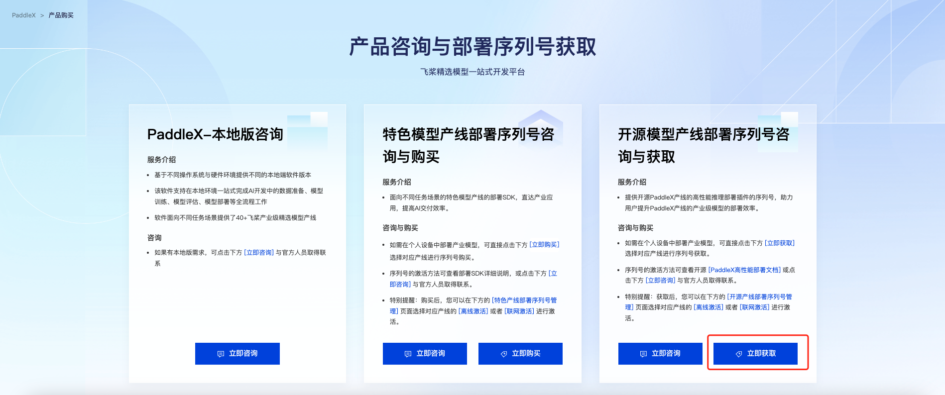
- 在 飞桨 AI Studio 星河社区-人工智能学习与实训社区 的“开源模型产线部署序列号咨询与获取”部分选择“立即获取”,如下图所示:
选择公式识别产线,并点击“获取”。之后,可以在页面下方的“开源产线部署SDK序列号管理”部分找到获取到的序列号:
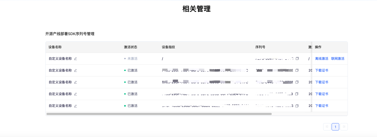
请注意:每个序列号只能绑定到唯一的设备指纹,且只能绑定一次。这意味着用户如果使用不同的机器部署产线,则必须为每台机器准备单独的序列号。
5.2.3 运行服务
运行服务:
-
支持使用 NVIDIA GPU 部署的镜像(机器上需要安装有支持 CUDA 11.8 的 NVIDIA 驱动):
-
CPU-only 镜像:
准备好镜像后,切换到 server 目录,执行如下命令运行服务器:
docker run \
    -it \
    -e PADDLEX_HPS_DEVICE_TYPE={部署设备类型} \
    -e PADDLEX_HPS_SERIAL_NUMBER={序列号} \
    -e PADDLEX_HPS_UPDATE_LICENSE=1 \
    -v "$(pwd)":/workspace \
    -v "${HOME}/.baidu/paddlex/licenses":/root/.baidu/paddlex/licenses \
    -v /dev/disk/by-uuid:/dev/disk/by-uuid \
    -w /workspace \
    --rm \
    --gpus all \
    --init \
    --network host \
    --shm-size 8g \
    {镜像名称} \
    /bin/bash server.sh
- 部署设备类型可以为
cpu或gpu,CPU-only 镜像仅支持cpu。 - 如果希望使用 CPU 部署,则不需要指定
--gpus。 -
以上命令必须在激活成功后才可以正常执行。PaddleX 提供两种激活方式:离线激活和在线激活。具体说明如下:
- 联网激活:在第一次执行时设置
PADDLEX_HPS_UPDATE_LICENSE为1,使程序自动更新证书并完成激活。再次执行命令时可以将PADDLEX_HPS_UPDATE_LICENSE设置为0以避免联网更新证书。 - 离线激活:按照序列号管理部分中的指引,获取机器的设备指纹,并将序列号与设备指纹绑定以获取证书,完成激活。使用这种激活方式,需要手动将证书存放在机器的
${HOME}/.baidu/paddlex/licenses目录中(如果目录不存在,需要创建目录)。使用这种方式时,将PADDLEX_HPS_UPDATE_LICENSE设置为0以避免联网更新证书。
- 联网激活:在第一次执行时设置
-
必须确保宿主机的
/dev/disk/by-uuid存在且非空,并正确挂载该目录,才能正常执行激活。 - 如果需要进入容器内部调试,可以将命令中的
/bin/bash server.sh替换为/bin/bash,然后在容器中执行/bin/bash server.sh。 - 如果希望服务器在后台运行,可以将命令中的
-it替换为-d。容器启动后,可通过docker logs -f {容器 ID}查看容器日志。 - 在命令中添加
-e PADDLEX_USE_HPIP=1可以使用 PaddleX 高性能推理插件加速产线推理过程。但请注意,并非所有产线都支持使用高性能推理插件。请参考 PaddleX 高性能推理指南 获取更多信息。
可观察到类似下面的输出信息:
I1216 11:37:21.601943 35 grpc_server.cc:4117] Started GRPCInferenceService at 0.0.0.0:8001
I1216 11:37:21.602333 35 http_server.cc:2815] Started HTTPService at 0.0.0.0:8000
I1216 11:37:21.643494 35 http_server.cc:167] Started Metrics Service at 0.0.0.0:8002
5.2.4 调用服务
目前,仅支持使用 Python 客户端调用服务。支持的 Python 版本为 3.8 至 3.12。
切换到高稳定性服务化部署 SDK 的 client 目录,执行如下命令安装依赖:
# 建议在虚拟环境中安装
python -m pip install -r requirements.txt
python -m pip install paddlex_hps_client-*.whl
client 目录的 client.py 脚本包含服务的调用示例,并提供命令行接口。
5.3 此外,PaddleX 也提供了其他三种部署方式,说明如下:
- 高性能部署:在实际生产环境中,许多应用对部署策略的性能指标(尤其是响应速度)有着较严苛的标准,以确保系统的高效运行与用户体验的流畅性。为此,PaddleX 提供高性能推理插件,旨在对模型推理及前后处理进行深度性能优化,实现端到端流程的显著提速,详细的高性能部署流程请参考 PaddleX 高性能推理指南。
- 基础服务化部署:服务化部署是实际生产环境中常见的一种部署形式。通过将推理功能封装为服务,客户端可以通过网络请求来访问这些服务,以获取推理结果。PaddleX 支持用户以低成本实现产线的服务化部署,详细的服务化部署流程请参考 PaddleX 服务化部署指南。
- 端侧部署:端侧部署是一种将计算和数据处理功能放在用户设备本身上的方式,设备可以直接处理数据,而不需要依赖远程的服务器。PaddleX 支持将模型部署在 Android 等端侧设备上,详细的端侧部署流程请参考 PaddleX端侧部署指南。
您可以根据需要选择合适的方式部署模型产线,进而进行后续的 AI 应用集成。