通用图像分类产线使用教程
1. 通用图像分类产线介绍
图像分类是一种将图像分配到预定义类别的技术。它广泛应用于物体识别、场景理解和自动标注等领域。图像分类可以识别各种物体,如动物、植物、交通标志等,并根据其特征将其归类。通过使用深度学习模型,图像分类能够自动提取图像特征并进行准确分类。本产线同时提供了灵活的服务化部署方式,支持在多种硬件上使用多种编程语言调用。不仅如此,本产线也提供了二次开发的能力,您可以基于本产线在您自己的数据集上训练调优,训练后的模型也可以无缝集成。
 通用图像分类产线中包含了图像分类模块,如您更考虑模型精度,请选择精度较高的模型,如您更考虑模型推理速度,请选择推理速度较快的模型,如您更考虑模型存储大小,请选择存储大小较小的模型。
推理耗时仅包含模型推理耗时,不包含前后处理耗时。
| 模型 | 模型下载链接 | Top1 Acc(%) | GPU推理耗时(ms) [常规模式 / 高性能模式] |
CPU推理耗时(ms) [常规模式 / 高性能模式] |
模型存储大小(MB) | 介绍 |
|---|---|---|---|---|---|---|
| CLIP_vit_base_patch16_224 | 推理模型/训练模型 | 85.36 | 12.03 / 2.49 | 60.86 / 42.69 | 331 | 视觉大模型 CLIP 在 ImageNet1k 数据集 fine-tune 的通用图像分类高精度模型 |
| MobileNetV3_small_x1_0 | 推理模型/训练模型 | 68.2 | 4.23 / 0.78 | 5.24 / 1.48 | 10.5 | MobileNetV3 是 Google 于 2019 年提出的一种基于 NAS 的新的轻量级网络,为了进一步提升效果,将 relu 和 sigmoid 激活函数分别替换为 hard_swish 与 hard_sigmoid 激活函数,同时引入了一些专门减小网络计算量的改进策略。 |
| PP-HGNet_small | 推理模型/训练模型 | 81.51 | 5.87 / 1.68 | 25.58 / 18.50 | 86.5 | PP-HGNet(High Performance GPU Net) 是百度飞桨视觉团队自研的更适用于 GPU 平台的高性能骨干网络,该网络在 VOVNet 的基础上使用了可学习的下采样层(LDS Layer),融合了 ResNet_vd、PPHGNet 等模型的优点,该模型在 GPU 平台上与其他 SOTA 模型在相同的速度下有着更高的精度。 |
| PP-HGNetV2-B0 | 推理模型/训练模型 | 77.77 | 4.41 / 0.87 | 10.58 / 1.87 | 21.4 | PP-HGNetV2(High Performance GPU Network V2) 是百度飞桨视觉团队自研的 PP-HGNet 的下一代版本,其在 PP-HGNet 的基础上,做了进一步优化和改进,最终在 NVIDIA GPU 设备上,将 "Accuracy-Latency Balance" 做到了极致,精度大幅超过了其他同样推理速度的模型。 |
| PP-HGNetV2-B4 | 推理模型/训练模型 | 83.57 | 7.05 / 1.16 | 16.23 / 7.55 | 70.4 | |
| PP-HGNetV2-B6 | 推理模型/训练模型 | 86.30 | 13.86 / 3.28 | 67.25 / 56.70 | 268.4 | |
| PP-LCNet_x1_0 | 推理模型/训练模型 | 71.32 | 2.59 / 0.68 | 3.18 / 1.19 | 10.5 | PP-LCNet_x1_0针对 Intel CPU 设备以及其加速库 MKLDNN 设计了特定的骨干网络,比起其他的轻量级的 SOTA 模型,该骨干网络可以在不增加推理时间的情况下,进一步提升模型的性能,最终大幅度超越现有的 SOTA 模型 |
| ResNet50 | 推理模型/训练模型 | 76.5 | 6.25 / 1.17 | 15.93 / 9.72 | 90.8 | ResNet 系列模型是在 2015 年提出的,一举在 ILSVRC2015 比赛中取得冠军,top5 错误率为 3.57%。该网络创新性的提出了残差结构,通过堆叠多个残差结构从而构建了 ResNet 网络。 |
| SwinTransformer_tiny_patch4_window7_224 | 推理模型/训练模型 | 81.10 | 7.11 / 2.01 | 62.72 / 47.35 | 100.1 | SwinTransformer 是一种新的视觉 Transformer 网络,可以用作计算机视觉领域的通用骨干网路。SwinTransformer 由移动窗口(shifted windows)表示的层次 Transformer 结构组成。移动窗口将自注意计算限制在非重叠的局部窗口上,同时允许跨窗口连接,从而提高了网络性能。 |
❗ 以上列出的是图像分类模块重点支持的9个核心模型,该模块总共支持80个模型,完整的模型列表如下:
👉模型列表详情
| 模型 | 模型下载链接 | Top1 Acc(%) | GPU推理耗时(ms) [常规模式 / 高性能模式] |
CPU推理耗时(ms) [常规模式 / 高性能模式] |
模型存储大小(MB) | 介绍 |
|---|---|---|---|---|---|---|
| CLIP_vit_base_patch16_224 | 推理模型/训练模型 | 85.36 | 12.03 / 2.49 | 60.86 / 42.69 | 331 | CLIP是一种基于视觉和语言相关联的图像分类模型,采用对比学习和预训练方法,实现无监督或弱监督的图像分类,尤其适用于大规模数据集。模型通过将图像和文本映射到同一表示空间,学习到通用特征,具有良好的泛化能力和解释性。其在较好的训练误差,在很多下游任务都有较好的表现。 |
| CLIP_vit_large_patch14_224 | 推理模型/训练模型 | 88.1 | 49.15 / 9.75 | 223.16 / 206.49 | 1040 | |
| ConvNeXt_base_224 | 推理模型/训练模型 | 83.84 | 11.37 / 5.65 | 143.98 / 52.31 | 313.9 | ConvNeXt系列模型是Meta在2022年提出的基于CNN架构的模型。该系列模型是在ResNet的基础上,通过借鉴SwinTransformer的优点设计,包括训练策略和网络结构的优化思路,从而改进的纯CNN架构网络,探索了卷积神经网络的性能上限。ConvNeXt系列模型具备卷积神经网络的诸多优点,包括推理效率高和易于迁移到下游任务等。 |
| ConvNeXt_base_384 | 推理模型/训练模型 | 84.90 | 29.48 / 11.17 | 293.76 / 134.27 | 313.9 | |
| ConvNeXt_large_224 | 推理模型/训练模型 | 84.26 | 22.99 / 12.73 | 220.79 / 113.24 | 700.7 | |
| ConvNeXt_large_384 | 推理模型/训练模型 | 85.27 | 58.90 / 24.63 | 509.48 / 260.27 | 700.7 | |
| ConvNeXt_small | 推理模型/训练模型 | 83.13 | 7.72 / 4.35 | 95.92 / 33.34 | 178.0 | |
| ConvNeXt_tiny | 推理模型/训练模型 | 82.03 | 6.00 / 2.47 | 63.59 / 18.23 | 104.1 | |
| FasterNet-L | 推理模型/训练模型 | 83.5 | 11.96 / 2.68 | 51.93 / 35.33 | 357.1 | FasterNet是一个旨在提高运行速度的神经网络,改进点主要如下: 1.重新审视了流行的运算符,发现低FLOPS主要来自于运算频繁的内存访问,特别是深度卷积; 2.提出了部分卷积(PConv),通过减少冗余计算和内存访问来更高效地提取图像特征; 3.基于PConv推出了FasterNet系列模型,这是一种新的设计方案,在不影响模型任务性能的情况下,在各种设备上实现了显著更高的运行速度。 |
| FasterNet-M | 推理模型/训练模型 | 83.0 | 11.17 / 2.16 | 38.49 / 21.17 | 204.6 | |
| FasterNet-S | 推理模型/训练模型 | 81.3 | 7.70 / 1.24 | 19.51 / 11.22 | 119.3 | |
| FasterNet-T0 | 推理模型/训练模型 | 71.9 | 4.73 / 0.82 | 6.40 / 1.96 | 15.1 | |
| FasterNet-T1 | 推理模型/训练模型 | 75.9 | 4.80 / 0.80 | 8.14 / 3.13 | 29.2 | |
| FasterNet-T2 | 推理模型/训练模型 | 79.1 | 6.10 / 0.88 | 12.71 / 5.35 | 57.4 | |
| MobileNetV1_x0_5 | 推理模型/训练模型 | 63.5 | 1.98 / 0.51 | 2.50 / 1.04 | 4.8 | MobileNetV1是Google于2017年发布的用于移动设备或嵌入式设备中的网络。该网络将传统的卷积操作拆解成深度可分离卷积,即Depthwise卷积和Pointwise卷积的组合。相比传统的卷积网络,该组合可以大大节省参数量和计算量。同时该网络可以用于图像分类等其他视觉任务中。 |
| MobileNetV1_x0_25 | 推理模型/训练模型 | 51.4 | 1.99 / 0.45 | 1.82 / 0.73 | 1.8 | |
| MobileNetV1_x0_75 | 推理模型/训练模型 | 68.8 | 2.33 / 0.41 | 3.33 / 1.34 | 9.3 | |
| MobileNetV1_x1_0 | 推理模型/训练模型 | 71.0 | 2.31 / 0.45 | 3.91 / 1.89 | 15.2 | |
| MobileNetV2_x0_5 | 推理模型/训练模型 | 65.0 | 3.58 / 0.62 | 3.86 / 1.23 | 7.1 | MobileNetV2是Google继MobileNetV1提出的一种轻量级网络。相比MobileNetV1,MobileNetV2提出了Linear bottlenecks与Inverted residual block作为网络基本结构,通过大量地堆叠这些基本模块,构成了MobileNetV2的网络结构。最后,在FLOPs只有MobileNetV1的一半的情况下取得了更高的分类精度。 |
| MobileNetV2_x0_25 | 推理模型/训练模型 | 53.2 | 3.05 / 0.66 | 3.30 / 0.98 | 5.5 | |
| MobileNetV2_x1_0 | 推理模型/训练模型 | 72.2 | 3.85 / 0.63 | 5.50 / 1.87 | 12.6 | |
| MobileNetV2_x1_5 | 推理模型/训练模型 | 74.1 | 3.93 / 0.73 | 8.84 / 3.12 | 25.0 | |
| MobileNetV2_x2_0 | 推理模型/训练模型 | 75.2 | 3.89 / 0.79 | 10.36 / 4.50 | 41.2 | |
| MobileNetV3_large_x0_5 | 推理模型/训练模型 | 69.2 | 4.60 / 0.77 | 5.32 / 1.58 | 9.6 | MobileNetV3是Google于2019年提出的一种基于NAS的轻量级网络。为了进一步提升效果,将relu和sigmoid激活函数分别替换为hard_swish与hard_sigmoid激活函数,同时引入了一些专门为减少网络计算量的改进策略。 |
| MobileNetV3_large_x0_35 | 推理模型/训练模型 | 64.3 | 4.44 / 0.75 | 5.20 / 1.50 | 7.5 | |
| MobileNetV3_large_x0_75 | 推理模型/训练模型 | 73.1 | 5.30 / 0.85 | 6.02 / 1.93 | 14.0 | |
| MobileNetV3_large_x1_0 | 推理模型/训练模型 | 75.3 | 5.38 / 0.81 | 7.16 / 2.19 | 19.5 | |
| MobileNetV3_large_x1_25 | 推理模型/训练模型 | 76.4 | 5.54 / 0.84 | 7.06 / 2.84 | 26.5 | |
| MobileNetV3_small_x0_5 | 推理模型/训练模型 | 59.2 | 3.87 / 0.77 | 4.90 / 1.32 | 6.8 | |
| MobileNetV3_small_x0_35 | 推理模型/训练模型 | 53.0 | 3.68 / 0.77 | 3.94 / 1.27 | 6.0 | |
| MobileNetV3_small_x0_75 | 推理模型/训练模型 | 66.0 | 3.92 / 0.77 | 4.68 / 1.39 | 8.5 | |
| MobileNetV3_small_x1_0 | 推理模型/训练模型 | 68.2 | 4.23 / 0.78 | 5.24 / 1.48 | 10.5 | |
| MobileNetV3_small_x1_25 | 推理模型/训练模型 | 70.7 | 4.59 / 0.79 | 5.36 / 1.63 | 13.0 | |
| MobileNetV4_conv_large | 推理模型/训练模型 | 83.4 | 9.04 / 2.28 | 34.34 / 22.01 | 125.2 | MobileNetV4是专为移动设备设计的高效架构。其核心在于引入了UIB(Universal Inverted Bottleneck)模块,这是一种统一且灵活的结构,融合了IB(Inverted Bottleneck)、ConvNeXt、FFN(Feed Forward Network)以及最新的ExtraDW(Extra Depthwise)模块。与UIB同时推出的还有Mobile MQA,这是种专为移动加速器定制的注意力块,可实现高达39%的显著加速。此外,MobileNetV4引入了一种新的神经架构搜索(Neural Architecture Search, NAS)方案,以提升搜索的有效性。 |
| MobileNetV4_conv_medium | 推理模型/训练模型 | 79.9 | 5.70 / 1.05 | 13.78 / 5.64 | 37.6 | |
| MobileNetV4_conv_small | 推理模型/训练模型 | 74.6 | 3.81 / 0.55 | 5.24 / 1.50 | 14.7 | |
| MobileNetV4_hybrid_large | 推理模型/训练模型 | 83.8 | 13.43 / 4.28 | 61.16 / 31.06 | 145.1 | |
| MobileNetV4_hybrid_medium | 推理模型/训练模型 | 80.5 | 11.82 / 1.30 | 22.01 / 6.06 | 42.9 | |
| PP-HGNet_base | 推理模型/训练模型 | 85.0 | 13.43 / 3.81 | 71.24 / 51.48 | 249.4 | PP-HGNet(High Performance GPU Net)是百度飞桨视觉团队研发的适用于GPU平台的高性能骨干网络。该网络结合VOVNet的基础出使用了可学习的下采样层(LDS Layer),融合了ResNet_vd、PPHGNet等模型的优点。该模型在GPU平台上与其他SOTA模型在相同的速度下有着更高的精度。在同等速度下,该模型高于ResNet34-0模型3.8个百分点,高于ResNet50-0模型2.4个百分点,在使用相同的SLSD条款下,最终超越了ResNet50-D模型4.7个百分点。与此同时,在相同精度下,其推理速度也远超主流VisionTransformer的推理速度。 |
| PP-HGNet_small | 推理模型/训练模型 | 81.51 | 5.87 / 1.68 | 25.58 / 18.50 | 86.5 | |
| PP-HGNet_tiny | 推理模型/训练模型 | 79.83 | 5.84 / 1.38 | 17.03 / 10.58 | 52.4 | |
| PP-HGNetV2-B0 | 推理模型/训练模型 | 77.77 | 4.41 / 0.87 | 10.58 / 1.87 | 21.4 | PP-HGNetV2(High Performance GPU Network V2)是百度飞桨视觉团队的PP-HGNet的下一代版本,其在PP-HGNet的基础上,做了进一步优化和改进,其在NVIDIA发布的“Accuracy-Latency Balance”做到了极致,精度大幅超越了其他同样推理速度的模型。在每种标签分类,考标场景中,都有较强的表现。 |
| PP-HGNetV2-B1 | 推理模型/训练模型 | 79.18 | 4.52 / 0.73 | 11.98 / 2.28 | 22.6 | |
| PP-HGNetV2-B2 | 推理模型/训练模型 | 81.74 | 6.67 / 0.96 | 14.22 / 4.04 | 39.9 | |
| PP-HGNetV2-B3 | 推理模型/训练模型 | 82.98 | 7.47 / 1.94 | 17.73 / 5.63 | 57.9 | |
| PP-HGNetV2-B4 | 推理模型/训练模型 | 83.57 | 7.05 / 1.16 | 16.23 / 7.55 | 70.4 | |
| PP-HGNetV2-B5 | 推理模型/训练模型 | 84.75 | 10.38 / 1.95 | 31.53 / 18.02 | 140.8 | |
| PP-HGNetV2-B6 | 推理模型/训练模型 | 86.30 | 13.86 / 3.28 | 67.25 / 56.70 | 268.4 | |
| PP-LCNet_x0_5 | 推理模型/训练模型 | 63.14 | 2.41 / 0.60 | 2.54 / 0.90 | 6.7 | PP-LCNet是百度飞桨视觉团队自研的轻量级骨干网络,它能在不增加推理时间的前提下,进一步提升模型的性能,大幅超越其他轻量级SOTA模型。 |
| PP-LCNet_x0_25 | 推理模型/训练模型 | 51.86 | 2.16 / 0.60 | 2.73 / 0.77 | 5.5 | |
| PP-LCNet_x0_35 | 推理模型/训练模型 | 58.09 | 2.18 / 0.60 | 2.32 / 0.89 | 5.9 | |
| PP-LCNet_x0_75 | 推理模型/训练模型 | 68.18 | 2.61 / 0.58 | 3.00 / 1.09 | 8.4 | |
| PP-LCNet_x1_0 | 推理模型/训练模型 | 71.32 | 2.59 / 0.68 | 3.18 / 1.19 | 10.5 | |
| PP-LCNet_x1_5 | 推理模型/训练模型 | 73.71 | 2.60 / 0.68 | 3.98 / 1.66 | 16.0 | |
| PP-LCNet_x2_0 | 推理模型/训练模型 | 75.18 | 2.53 / 0.68 | 5.21 / 2.24 | 23.2 | |
| PP-LCNet_x2_5 | 推理模型/训练模型 | 76.60 | 2.76 / 0.67 | 6.78 / 3.20 | 32.1 | |
| PP-LCNetV2_base | 推理模型/训练模型 | 77.05 | 4.04 / 0.62 | 6.80 / 2.67 | 23.7 | PP-LCNetV2 图像分类模型是百度飞桨视觉团队自研的 PP-LCNet 的下一代版本,其在 PP-LCNet 的基础上,做了进一步优化和改进,主要使用重参数化策略组合了不同大小卷积核的深度卷积,并优化了点卷积、Shortcut等。在不使用额外数据的前提下,PPLCNetV2_base 模型在图像分类 ImageNet 数据集上能够取得超过 77% 的 Top1 Acc,同时在 Intel CPU 平台的推理时间在 4.4 ms 以下 |
| PP-LCNetV2_large | 推理模型/训练模型 | 78.51 | 4.91 / 0.85 | 10.30 / 5.38 | 37.3 | |
| PP-LCNetV2_small | 推理模型/训练模型 | 73.97 | 3.07 / 0.60 | 4.28 / 1.58 | 14.6 | |
| ResNet18_vd | 推理模型/训练模型 | 72.3 | 2.87 / 0.77 | 7.91 / 4.64 | 41.5 | ResNet 系列模型是在 2015 年提出的,一举在 ILSVRC2015 比赛中取得冠军,top5 错误率为 3.57%。该网络创新性的提出了残差结构,通过堆叠多个残差结构从而构建了 ResNet 网络。实验表明使用残差块可以有效地提升收敛速度和精度。 |
| ResNet18 | 推理模型/训练模型 | 71.0 | 2.63 / 0.74 | 6.30 / 4.16 | 41.5 | |
| ResNet34_vd | 推理模型/训练模型 | 76.0 | 4.47 / 1.09 | 14.30 / 8.33 | 77.3 | |
| ResNet34 | 推理模型/训练模型 | 74.6 | 4.20 / 1.07 | 12.53 / 7.83 | 77.3 | |
| ResNet50_vd | 推理模型/训练模型 | 79.1 | 6.66 / 1.23 | 16.34 / 10.00 | 90.8 | |
| ResNet50 | 推理模型/训练模型 | 76.5 | 6.25 / 1.17 | 15.93 / 9.72 | 90.8 | |
| ResNet101_vd | 推理模型/训练模型 | 80.2 | 11.93 / 2.07 | 32.47 / 23.62 | 158.4 | |
| ResNet101 | 推理模型/训练模型 | 77.6 | 13.73 / 2.06 | 29.69 / 17.72 | 158.4 | |
| ResNet152_vd | 推理模型/训练模型 | 80.6 | 20.70 / 2.82 | 43.90 / 27.91 | 214.3 | |
| ResNet152 | 推理模型/训练模型 | 78.3 | 17.86 / 2.79 | 46.19 / 26.00 | 214.2 | |
| ResNet200_vd | 推理模型/训练模型 | 80.9 | 22.55 / 3.54 | 58.54 / 35.70 | 266.0 | |
| StarNet-S1 | 推理模型/训练模型 | 73.6 | 6.24 / 0.96 | 8.78 / 2.44 | 11.2 | StarNet 聚焦于研究网络设计中“星操作”(即元素级乘法)的未开发潜力。揭示星操作能够将输入映射到高维、非线性特征空间的能力,这一过程类似于核技巧,但无需扩大网络规模。因此进一步提出了 StarNet,一个简单而强大的原型网络,该网络在紧凑的网络结构和有限的计算资源下,展现出了卓越的性能和低延迟。 |
| StarNet-S2 | 推理模型/训练模型 | 74.8 | 4.78 / 0.85 | 7.24 / 2.48 | 14.3 | |
| StarNet-S3 | 推理模型/训练模型 | 77.0 | 6.77 / 1.07 | 9.69 / 3.35 | 22.2 | |
| StarNet-S4 | 推理模型/训练模型 | 79.0 | 9.01 / 1.48 | 14.79 / 4.58 | 28.9 | |
| SwinTransformer_base_patch4_window7_224 | 推理模型/训练模型 | 83.37 | 13.04 / 10.77 | 133.79 / 118.45 | 340 | SwinTransformer 是一种新的视觉 Transformer 网络,可以用作计算机视觉领域的通用骨干网路。SwinTransformer 由移动窗口(shifted windows)表示的层次 Transformer 结构组成。移动窗口将自注意计算限制在非重叠的局部窗口上,同时允许跨窗口连接,从而提高了网络性能。 |
| SwinTransformer_base_patch4_window12_384 | 推理模型/训练模型 | 84.17 | 33.99 / 28.42 | 400.19 / 317.36 | 311.4 | |
| SwinTransformer_large_patch4_window7_224 | 推理模型/训练模型 | 86.19 | 23.69 / 6.18 | 198.60 / 177.18 | 694.8 | |
| SwinTransformer_large_patch4_window12_384 | 推理模型/训练模型 | 87.06 | 68.07 / 14.84 | 609.07 / 525.72 | 696.1 | |
| SwinTransformer_small_patch4_window7_224 | 推理模型/训练模型 | 83.21 | 12.17 / 3.51 | 111.03 / 92.51 | 175.6 | |
| SwinTransformer_tiny_patch4_window7_224 | 推理模型/训练模型 | 81.10 | 7.11 / 2.01 | 62.72 / 47.35 | 100.1 |
- 性能测试环境
- 测试数据集: ImageNet-1k 验证集。
- 硬件配置:
- GPU:NVIDIA Tesla T4
- CPU:Intel Xeon Gold 6271C @ 2.60GHz
- 软件环境:
- Ubuntu 20.04 / CUDA 11.8 / cuDNN 8.9 / TensorRT 8.6.1.6
- paddlepaddle 3.0.0 / paddlex 3.0.3
- 推理模式说明
| 模式 | GPU配置 | CPU配置 | 加速技术组合 |
|---|---|---|---|
| 常规模式 | FP32精度 / 无TRT加速 | FP32精度 / 8线程 | PaddleInference |
| 高性能模式 | 选择先验精度类型和加速策略的最优组合 | FP32精度 / 8线程 | 选择先验最优后端(Paddle/OpenVINO/TRT等) |
2. 快速开始
PaddleX 所提供的模型产线均可以快速体验效果,你可以在星河社区线体验通用图像分类产线的效果,也可以在本地使用命令行或 Python 体验通用图像分类产线的效果。
2.1 在线体验
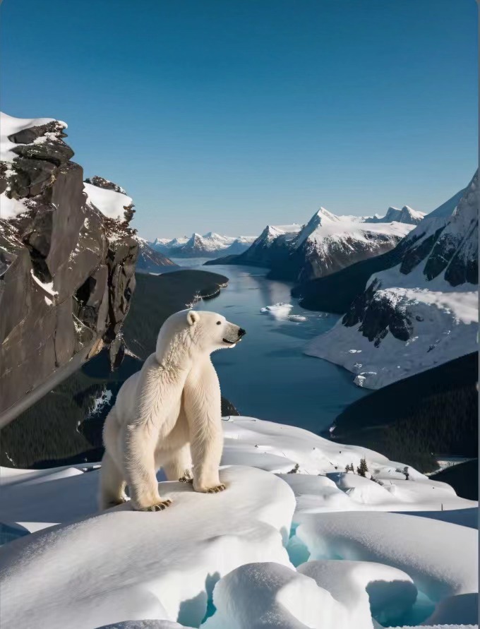
您可以在线体验通用图像分类产线的效果,用官方提供的 demo 图片进行识别,例如:

如果您对产线运行的效果满意,可以直接进行集成部署。您可以选择从云端下载部署包,也可以参考2.2节本地体验中的方法进行本地部署。如果对效果不满意,您可以利用私有数据对产线中的模型进行微调训练。如果您具备本地训练的硬件资源,可以直接在本地开展训练;如果没有,星河零代码平台提供了一键式训练服务,无需编写代码,只需上传数据后,即可一键启动训练任务。
2.2 本地体验
在本地使用通用图像分类产线前,请确保您已经按照PaddleX本地安装教程完成了PaddleX的wheel包安装。如果您希望选择性安装依赖,请参考安装教程中的相关说明。该产线对应的依赖分组为 cv。
2.2.1 命令行方式体验
一行命令即可快速体验图像分类产线效果,使用 测试文件,并将 --input 替换为本地路径,进行预测
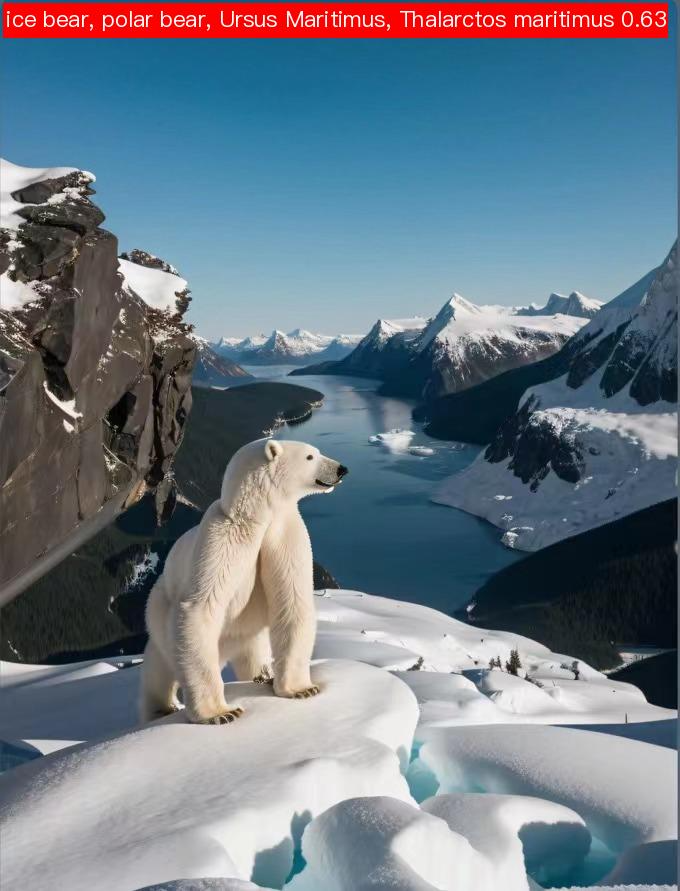
paddlex --pipeline image_classification --input general_image_classification_001.jpg --device gpu:0 --save_path ./output/
运行后,会将结果打印到终端上,结果如下:
{'res': {'input_path': 'general_image_classification_001.jpg', 'page_index': None, 'class_ids': array([296, 170, 356, 258, 248], dtype=int32), 'scores': array([0.62736, 0.03752, 0.03256, 0.0323 , 0.03194], dtype=float32), 'label_names': ['ice bear, polar bear, Ursus Maritimus, Thalarctos maritimus', 'Irish wolfhound', 'weasel', 'Samoyed, Samoyede', 'Eskimo dog, husky']}}
运行结果参数说明可以参考2.2.2 Python脚本方式集成中的结果解释。
可视化结果保存在save_path下,其中图像分类的可视化结果如下:
2.2.2 Python脚本方式集成
- 上述命令行是为了快速体验查看效果,一般来说,在项目中,往往需要通过代码集成,您可以通过几行代码即可完成产线的快速推理,推理代码如下:
from paddlex import create_pipeline

pipeline = create_pipeline(pipeline="image_classification")

output = pipeline.predict("general_image_classification_001.jpg")
for res in output:
    res.print() ## 打印预测的结构化输出
    res.save_to_img(save_path="./output/") ## 保存结果可视化图像
    res.save_to_json(save_path="./output/") ## 保存预测的结构化输出
在上述 Python 脚本中,执行了如下几个步骤:
(1)通过 create_pipeline() 实例化通用图像分类产线对象,具体参数说明如下:
| 参数 | 参数说明 | 参数类型 | 默认值 | |
|---|---|---|---|---|
pipeline |
产线名称或是产线配置文件路径。如为产线名称,则必须为 PaddleX 所支持的产线。 | str |
None | |
config |
产线具体的配置信息(如果和pipeline同时设置,优先级高于pipeline,且要求产线名和pipeline一致)。 |
dict[str, Any] |
None |
|
device |
产线推理设备。支持指定GPU具体卡号,如“gpu:0”,其他硬件具体卡号,如“npu:0”,CPU如“cpu”。支持同时指定多个设备以进行并行推理,详情请参考产线并行推理文档。 | str |
gpu:0 |
|
use_hpip |
是否启用高性能推理插件。如果为 None,则使用配置文件或 config 中的配置。 |
bool | None |
无 | None |
hpi_config |
高性能推理配置 | dict | None |
无 | None |
(2)调用图像分类产线对象的 predict() 方法进行推理预测。该方法将返回一个 generator。以下是 predict() 方法的参数及其说明:
| 参数 | 参数说明 | 参数类型 | 可选项 | 默认值 |
|---|---|---|---|---|
input |
待预测数据,支持多种输入类型,必填 | Python Var|str|list |
|
None |
topk |
预测结果的前topk值,如果不指定,将默认使用PaddleX官方模型配置 |
int |
|
5 |
(3)对预测结果进行处理,每个样本的预测结果均为对应的Result对象,且支持打印、保存为图片、保存为json文件的操作:
| 方法 | 方法说明 | 参数 | 参数类型 | 参数说明 | 默认值 |
|---|---|---|---|---|---|
print() |
打印结果到终端 | format_json |
bool |
是否对输出内容进行使用 JSON 缩进格式化 |
True |
indent |
int |
指定缩进级别,以美化输出的 JSON 数据,使其更具可读性,仅当 format_json 为 True 时有效 |
4 | ||
ensure_ascii |
bool |
控制是否将非 ASCII 字符转义为 Unicode。设置为 True 时,所有非 ASCII 字符将被转义;False 则保留原始字符,仅当format_json为True时有效 |
False |
||
save_to_json() |
将结果保存为json格式的文件 | save_path |
str |
保存的文件路径,当为目录时,保存文件命名与输入文件类型命名一致 | 无 |
indent |
int |
指定缩进级别,以美化输出的 JSON 数据,使其更具可读性,仅当 format_json 为 True 时有效 |
4 | ||
ensure_ascii |
bool |
控制是否将非 ASCII 字符转义为 Unicode。设置为 True 时,所有非 ASCII 字符将被转义;False 则保留原始字符,仅当format_json为True时有效 |
False |
||
save_to_img() |
将结果保存为图像格式的文件 | save_path |
str |
保存的文件路径,支持目录或文件路径 | 无 |
-
调用
print()方法会将结果打印到终端,打印到终端的内容解释如下:input_path:(str)待预测图像的输入路径。page_index:(Union[int, None])如果输入是PDF文件,则表示当前是PDF的第几页,否则为Noneclass_ids:(List[numpy.ndarray])表示预测结果的类别id。scores:(List[numpy.ndarray])表示预测结果的置信度。label_names:(List[str])表示预测结果的类别名称。
-
调用
save_to_json()方法会将上述内容保存到指定的save_path中,如果指定为目录,则保存的路径为save_path/{your_img_basename}_res.json,如果指定为文件,则直接保存到该文件中。由于json文件不支持保存numpy数组,因此会将其中的numpy.array类型转换为列表形式。 -
调用
save_to_img()方法会将可视化结果保存到指定的save_path中,如果指定为目录,则保存的路径为save_path/{your_img_basename}_res.{your_img_extension},如果指定为文件,则直接保存到该文件中。(产线通常包含较多结果图片,不建议直接指定为具体的文件路径,否则多张图会被覆盖,仅保留最后一张图) -
此外,也支持通过属性获取带结果的可视化图像和预测结果,具体如下:
| 属性 | 属性说明 |
|---|---|
json |
获取预测的 json 格式的结果 |
img |
获取格式为 dict 的可视化图像 |
json属性获取的预测结果为dict类型的数据,相关内容与调用save_to_json()方法保存的内容一致。img属性返回的预测结果是一个字典类型的数据。其中,键为res对应的值是Image.Image对象:一个用于显示分类结果的可视化图像。
此外,您可以获取图像分类产线配置文件,并加载配置文件进行预测。可执行如下命令将结果保存在 my_path 中:
若您获取了配置文件,即可对通用图像分类产线各项配置进行自定义,只需要修改 create_pipeline 方法中的 pipeline 参数值为产线配置文件路径即可。示例如下:
from paddlex import create_pipeline

pipeline = create_pipeline(pipeline="./my_path/image_classification.yaml")

output = pipeline.predict(
    input="./general_image_classification_001.jpg",
)
for res in output:
    res.print()
    res.save_to_img("./output/")
    res.save_to_json("./output/")
注: 配置文件中的参数为产线初始化参数,如果希望更改通用图像分类产线初始化参数,可以直接修改配置文件中的参数,并加载配置文件进行预测。同时,CLI 预测也支持传入配置文件,--pipeline 指定配置文件的路径即可。
3. 开发集成/部署
如果产线可以达到您对产线推理速度和精度的要求,您可以直接进行开发集成/部署。
若您需要将产线直接应用在您的Python项目中,可以参考 2.2.2 Python脚本方式中的示例代码。
此外,PaddleX 也提供了其他三种部署方式,详细说明如下:
🚀 高性能推理:在实际生产环境中,许多应用对部署策略的性能指标(尤其是响应速度)有着较严苛的标准,以确保系统的高效运行与用户体验的流畅性。为此,PaddleX 提供高性能推理插件,旨在对模型推理及前后处理进行深度性能优化,实现端到端流程的显著提速,详细的高性能推理流程请参考PaddleX高性能推理指南。
☁️ 服务化部署:服务化部署是实际生产环境中常见的一种部署形式。通过将推理功能封装为服务,客户端可以通过网络请求来访问这些服务,以获取推理结果。PaddleX 支持多种产线服务化部署方案,详细的产线服务化部署流程请参考PaddleX服务化部署指南。
以下是基础服务化部署的API参考与多语言服务调用示例:
API参考
对于服务提供的主要操作:
- HTTP请求方法为POST。
- 请求体和响应体均为JSON数据(JSON对象)。
- 当请求处理成功时,响应状态码为
200,响应体的属性如下:
| 名称 | 类型 | 含义 |
|---|---|---|
logId |
string |
请求的UUID。 |
errorCode |
integer |
错误码。固定为0。 |
errorMsg |
string |
错误说明。固定为"Success"。 |
result |
object |
操作结果。 |
- 当请求处理未成功时,响应体的属性如下:
| 名称 | 类型 | 含义 |
|---|---|---|
logId |
string |
请求的UUID。 |
errorCode |
integer |
错误码。与响应状态码相同。 |
errorMsg |
string |
错误说明。 |
服务提供的主要操作如下:
infer
对图像进行分类。
POST /image-classification
- 请求体的属性如下:
| 名称 | 类型 | 含义 | 是否必填 |
|---|---|---|---|
image |
string |
服务器可访问的图像文件的URL或图像文件内容的Base64编码结果。 | 是 |
topk |
integer | null |
请参阅产线对象中 predict 方法的 topk 参数相关说明。 |
否 |
visualize |
boolean | null |
是否返回可视化结果图以及处理过程中的中间图像等。
例如,在产线配置文件中添加如下字段: visualize参数可以覆盖默认行为。如果请求体和配置文件中均未设置(或请求体传入null、配置文件中未设置),则默认返回图像。
|
否 |
- 请求处理成功时,响应体的
result具有如下属性:
| 名称 | 类型 | 含义 |
|---|---|---|
categories |
array |
图像类别信息。 |
image |
string | null |
图像分类结果图。图像为JPEG格式,使用Base64编码。 |
categories中的每个元素为一个object,具有如下属性:
| 名称 | 类型 | 含义 |
|---|---|---|
id |
integer |
类别ID。 |
name |
string |
类别名称。 |
score |
number |
类别得分。 |
result示例如下:
{
"categories": [
{
"id": 5,
"name": "兔子",
"score": 0.93
}
],
"image": "xxxxxx"
}
多语言调用服务示例
Python
import base64
import requests

API_URL = "http://localhost:8080/image-classification" # 服务URL
image_path = "./demo.jpg"
output_image_path = "./out.jpg"

# 对本地图像进行Base64编码
with open(image_path, "rb") as file:
    image_bytes = file.read()
    image_data = base64.b64encode(image_bytes).decode("ascii")

payload = {"image": image_data}  # Base64编码的文件内容或者图像URL

# 调用API
response = requests.post(API_URL, json=payload)

# 处理接口返回数据
assert response.status_code == 200
result = response.json()["result"]
with open(output_image_path, "wb") as file:
    file.write(base64.b64decode(result["image"]))
print(f"Output image saved at {output_image_path}")
print("\nCategories:")
print(result["categories"])
C++
#include <iostream>
#include "cpp-httplib/httplib.h" // https://github.com/Huiyicc/cpp-httplib
#include "nlohmann/json.hpp" // https://github.com/nlohmann/json
#include "base64.hpp" // https://github.com/tobiaslocker/base64

int main() {
    httplib::Client client("localhost:8080");
    const std::string imagePath = "./demo.jpg";
    const std::string outputImagePath = "./out.jpg";

    httplib::Headers headers = {
        {"Content-Type", "application/json"}
    };

    // 对本地图像进行Base64编码
    std::ifstream file(imagePath, std::ios::binary | std::ios::ate);
    std::streamsize size = file.tellg();
    file.seekg(0, std::ios::beg);

    std::vector<char> buffer(size);
    if (!file.read(buffer.data(), size)) {
        std::cerr << "Error reading file." << std::endl;
        return 1;
    }
    std::string bufferStr(reinterpret_cast<const char*>(buffer.data()), buffer.size());
    std::string encodedImage = base64::to_base64(bufferStr);

    nlohmann::json jsonObj;
    jsonObj["image"] = encodedImage;
    std::string body = jsonObj.dump();

    // 调用API
    auto response = client.Post("/image-classification", headers, body, "application/json");
    // 处理接口返回数据
    if (response && response->status == 200) {
        nlohmann::json jsonResponse = nlohmann::json::parse(response->body);
        auto result = jsonResponse["result"];

        encodedImage = result["image"];
        std::string decodedString = base64::from_base64(encodedImage);
        std::vector<unsigned char> decodedImage(decodedString.begin(), decodedString.end());
        std::ofstream outputImage(outPutImagePath, std::ios::binary | std::ios::out);
        if (outputImage.is_open()) {
            outputImage.write(reinterpret_cast<char*>(decodedImage.data()), decodedImage.size());
            outputImage.close();
            std::cout << "Output image saved at " << outPutImagePath << std::endl;
        } else {
            std::cerr << "Unable to open file for writing: " << outPutImagePath << std::endl;
        }

        auto categories = result["categories"];
        std::cout << "\nCategories:" << std::endl;
        for (const auto& category : categories) {
            std::cout << category << std::endl;
        }
    } else {
        std::cout << "Failed to send HTTP request." << std::endl;
        return 1;
    }

    return 0;
}
Java
import okhttp3.*;
import com.fasterxml.jackson.databind.ObjectMapper;
import com.fasterxml.jackson.databind.JsonNode;
import com.fasterxml.jackson.databind.node.ObjectNode;

import java.io.File;
import java.io.FileOutputStream;
import java.io.IOException;
import java.util.Base64;

public class Main {
    public static void main(String[] args) throws IOException {
        String API_URL = "http://localhost:8080/image-classification"; // 服务URL
        String imagePath = "./demo.jpg"; // 本地图像
        String outputImagePath = "./out.jpg"; // 输出图像

        // 对本地图像进行Base64编码
        File file = new File(imagePath);
        byte[] fileContent = java.nio.file.Files.readAllBytes(file.toPath());
        String imageData = Base64.getEncoder().encodeToString(fileContent);

        ObjectMapper objectMapper = new ObjectMapper();
        ObjectNode params = objectMapper.createObjectNode();
        params.put("image", imageData); // Base64编码的文件内容或者图像URL

        // 创建 OkHttpClient 实例
        OkHttpClient client = new OkHttpClient();
        MediaType JSON = MediaType.Companion.get("application/json; charset=utf-8");
        RequestBody body = RequestBody.Companion.create(params.toString(), JSON);
        Request request = new Request.Builder()
                .url(API_URL)
                .post(body)
                .build();

        // 调用API并处理接口返回数据
        try (Response response = client.newCall(request).execute()) {
            if (response.isSuccessful()) {
                String responseBody = response.body().string();
                JsonNode resultNode = objectMapper.readTree(responseBody);
                JsonNode result = resultNode.get("result");
                String base64Image = result.get("image").asText();
                JsonNode categories = result.get("categories");

                byte[] imageBytes = Base64.getDecoder().decode(base64Image);
                try (FileOutputStream fos = new FileOutputStream(outputImagePath)) {
                    fos.write(imageBytes);
                }
                System.out.println("Output image saved at " + outputImagePath);
                System.out.println("\nCategories: " + categories.toString());
            } else {
                System.err.println("Request failed with code: " + response.code());
            }
        }
    }
}
Go
package main

import (
    "bytes"
    "encoding/base64"
    "encoding/json"
    "fmt"
    "io/ioutil"
    "net/http"
)

func main() {
    API_URL := "http://localhost:8080/image-classification"
    imagePath := "./demo.jpg"
    outputImagePath := "./out.jpg"

    // 对本地图像进行Base64编码
    imageBytes, err := ioutil.ReadFile(imagePath)
    if err != nil {
        fmt.Println("Error reading image file:", err)
        return
    }
    imageData := base64.StdEncoding.EncodeToString(imageBytes)

    payload := map[string]string{"image": imageData} // Base64编码的文件内容或者图像URL
    payloadBytes, err := json.Marshal(payload)
    if err != nil {
        fmt.Println("Error marshaling payload:", err)
        return
    }

    // 调用API
    client := &http.Client{}
    req, err := http.NewRequest("POST", API_URL, bytes.NewBuffer(payloadBytes))
    if err != nil {
        fmt.Println("Error creating request:", err)
        return
    }

    res, err := client.Do(req)
    if err != nil {
        fmt.Println("Error sending request:", err)
        return
    }
    defer res.Body.Close()

    // 处理接口返回数据
    body, err := ioutil.ReadAll(res.Body)
    if err != nil {
        fmt.Println("Error reading response body:", err)
        return
    }
    type Response struct {
        Result struct {
            Image      string   `json:"image"`
            Categories []map[string]interface{} `json:"categories"`
        } `json:"result"`
    }
    var respData Response
    err = json.Unmarshal([]byte(string(body)), &respData)
    if err != nil {
        fmt.Println("Error unmarshaling response body:", err)
        return
    }

    outputImageData, err := base64.StdEncoding.DecodeString(respData.Result.Image)
    if err != nil {
        fmt.Println("Error decoding base64 image data:", err)
        return
    }
    err = ioutil.WriteFile(outputImagePath, outputImageData, 0644)
    if err != nil {
        fmt.Println("Error writing image to file:", err)
        return
    }
    fmt.Printf("Image saved at %s.jpg\n", outputImagePath)
    fmt.Println("\nCategories:")
    for _, category := range respData.Result.Categories {
        fmt.Println(category)
    }
}
C#
using System;
using System.IO;
using System.Net.Http;
using System.Net.Http.Headers;
using System.Text;
using System.Threading.Tasks;
using Newtonsoft.Json.Linq;

class Program
{
    static readonly string API_URL = "http://localhost:8080/image-classification";
    static readonly string imagePath = "./demo.jpg";
    static readonly string outputImagePath = "./out.jpg";

    static async Task Main(string[] args)
    {
        var httpClient = new HttpClient();

        // 对本地图像进行Base64编码
        byte[] imageBytes = File.ReadAllBytes(imagePath);
        string image_data = Convert.ToBase64String(imageBytes);

        var payload = new JObject{ { "image", image_data } }; // Base64编码的文件内容或者图像URL
        var content = new StringContent(payload.ToString(), Encoding.UTF8, "application/json");

        // 调用API
        HttpResponseMessage response = await httpClient.PostAsync(API_URL, content);
        response.EnsureSuccessStatusCode();

        // 处理接口返回数据
        string responseBody = await response.Content.ReadAsStringAsync();
        JObject jsonResponse = JObject.Parse(responseBody);

        string base64Image = jsonResponse["result"]["image"].ToString();
        byte[] outputImageBytes = Convert.FromBase64String(base64Image);

        File.WriteAllBytes(outputImagePath, outputImageBytes);
        Console.WriteLine($"Output image saved at {outputImagePath}");
        Console.WriteLine("\nCategories:");
        Console.WriteLine(jsonResponse["result"]["categories"].ToString());
    }
}
Node.js
const axios = require('axios');
const fs = require('fs');

const API_URL = 'http://localhost:8080/image-classification'
const imagePath = './demo.jpg'
const outputImagePath = "./out.jpg";

let config = {
   method: 'POST',
   maxBodyLength: Infinity,
   url: API_URL,
   data: JSON.stringify({
    'image': encodeImageToBase64(imagePath)  // Base64编码的文件内容或者图像URL
  })
};

// 对本地图像进行Base64编码
function encodeImageToBase64(filePath) {
  const bitmap = fs.readFileSync(filePath);
  return Buffer.from(bitmap).toString('base64');
}

// 调用API
axios.request(config)
.then((response) => {
    // 处理接口返回数据
    const result = response.data["result"];
    const imageBuffer = Buffer.from(result["image"], 'base64');
    fs.writeFile(outputImagePath, imageBuffer, (err) => {
      if (err) throw err;
      console.log(`Output image saved at ${outputImagePath}`);
    });
    console.log("\nCategories:");
    console.log(result["categories"]);
})
.catch((error) => {
  console.log(error);
});
PHP
<?php

$API_URL = "http://localhost:8080/image-classification"; // 服务URL
$image_path = "./demo.jpg";
$output_image_path = "./out.jpg";

// 对本地图像进行Base64编码
$image_data = base64_encode(file_get_contents($image_path));
$payload = array("image" => $image_data); // Base64编码的文件内容或者图像URL

// 调用API
$ch = curl_init($API_URL);
curl_setopt($ch, CURLOPT_POST, true);
curl_setopt($ch, CURLOPT_POSTFIELDS, json_encode($payload));
curl_setopt($ch, CURLOPT_HTTPHEADER, array('Content-Type: application/json'));
curl_setopt($ch, CURLOPT_RETURNTRANSFER, true);
$response = curl_exec($ch);
curl_close($ch);

// 处理接口返回数据
$result = json_decode($response, true)["result"];
file_put_contents($output_image_path, base64_decode($result["image"]));
echo "Output image saved at " . $output_image_path . "\n";
echo "\nCategories:\n";
print_r($result["categories"]);
?>
📱 端侧部署:端侧部署是一种将计算和数据处理功能放在用户设备本身上的方式,设备可以直接处理数据,而不需要依赖远程的服务器。PaddleX 支持将模型部署在 Android 等端侧设备上,详细的端侧部署流程请参考PaddleX端侧部署指南。 您可以根据需要选择合适的方式部署模型产线,进而进行后续的 AI 应用集成。
4. 二次开发
如果通用图像分类产线提供的默认模型权重在您的场景中,精度或速度不满意,您可以尝试利用您自己拥有的特定领域或应用场景的数据对现有模型进行进一步的微调,以提升通用图像分类产线的在您的场景中的识别效果。
4.1 模型微调
由于通用图像分类产线包含图像图像分类模块,如果模型产线的效果不及预期,需要参考以下表格中对应的微调教程链接进行模型微调。
| 情形 | 微调模块 | 微调参考链接 |
|---|---|---|
| 多标签分类效果不准 | 多标签分类模块 | 链接 |
4.2 模型应用
当您使用私有数据集完成微调训练后,可获得本地模型权重文件。
若您需要使用微调后的模型权重,只需对产线配置文件做修改,将微调后模型权重的本地路径替换至产线配置文件中的对应位置即可:
SubModules:
  ImageClassification:
    module_name: image_classification
    model_name: PP-LCNet_x0_5
    model_dir: null # 替换为微调后的图像分类模型权重路径
    batch_size: 4
    topk: 5
5. 多硬件支持
PaddleX 支持英伟达 GPU、昆仑芯 XPU、昇腾 NPU和寒武纪 MLU 等多种主流硬件设备,仅需修改 --device参数即可完成不同硬件之间的无缝切换。
例如,您使用昇腾 NPU 进行通用图像分类产线的推理,使用的 CLI 命令为:
paddlex --pipeline image_classification \
        --input general_image_classification_001.jpg \
        --save_path ./output \
        --device npu:0
当然,您也可以在 Python 脚本中 create_pipeline() 时或者 predict() 时指定硬件设备。
若您想在更多种类的硬件上使用通用图像分类产线,请参考PaddleX多硬件使用指南。