PaddleX 3.0 General Object Detection Pipeline — Tutorial for Fashion Element Detection
PaddleX offers a rich set of pipelines, each consisting of one or more models tailored to solve specific scenario tasks. All PaddleX pipelines support quick trials, and if the results are not satisfactory, you can fine-tune the models with your private data. PaddleX also provides Python APIs for easy integration into personal projects. Before proceeding, ensure you have installed PaddleX. For installation instructions, refer to PaddleX Installation. This tutorial introduces the usage of the pipeline tool with an example of fashion element detection in clothing.
1. Select a Pipeline
First, choose the corresponding PaddleX pipeline based on your task scenario. For fashion element detection, this falls under the General Object Detection pipeline in PaddleX. If unsure about the task-pipeline correspondence, consult the Pipeline List for capabilities of each pipeline.
2. Quick Start
PaddleX offers two ways to experience the pipeline: locally through the PaddleX wheel package or on the Baidu AIStudio Community.
-
Local Experience:
-
AIStudio Community Experience: Visit Baidu AIStudio Community, click "Create Pipeline," and select the General Object Detection pipeline for a quick trial.
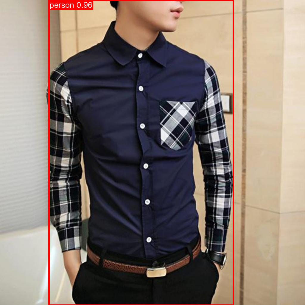
Quick Trial Output Example:

After the trial, determine if the pipeline meets your expectations (including accuracy, speed, etc.). If the model's speed or accuracy is unsatisfactory, test alternative models or proceed with fine-tuning. For this tutorial, aiming to detect fashion elements in clothing, the default weights (trained on the COCO dataset) are insufficient. Data collection and annotation, followed by training and fine-tuning, are necessary.
3. Choose a Model
PaddleX provides 37 end-to-end object detection models. Refer to the Model List for details. Below are benchmarks for some models:
| Model List | mAP(%) | GPU Inference Time(ms) | CPU Inference Time(ms) | Model Size(M) |
|---|---|---|---|---|
| RT-DETR-H | 56.3 | 100.65 | 8451.92 | 471 |
| RT-DETR-L | 53.0 | 27.89 | 841.00 | 125 |
| PP-YOLOE_plus-L | 52.9 | 29.67 | 700.97 | 200 |
| PP-YOLOE_plus-S | 43.7 | 8.11 | 137.23 | 31 |
| PicoDet-L | 42.6 | 10.09 | 129.32 | 23 |
| PicoDet-S | 29.1 | 3.17 | 13.36 | 5 |
Note: The above accuracy metrics are mAP(0.5:0.95) on the COCO2017 validation set. GPU inference time is based on an NVIDIA Tesla T4 machine with FP32 precision. CPU inference speed is based on an Intel(R) Xeon(R) Gold 5117 CPU @ 2.00GHz with 8 threads and FP32 precision.
In summary, models with faster inference speed are placed higher in the table, while models with higher accuracy are lower. This tutorial takes the PicoDet-L model as an example to complete a full model development process. You can judge and select an appropriate model for training based on your actual usage scenarios. After training, you can evaluate the suitable model weights within the pipeline and ultimately use them in practical scenarios.
4. Data Preparation and Verification
4.1 Data Preparation
This tutorial uses the "Fashion Element Detection Dataset" as an example dataset. You can obtain the example dataset using the following commands. If you use your own annotated dataset, you need to adjust it according to PaddleX's format requirements to meet PaddleX's data format specifications. For data format introductions, you can refer to the PaddleX Object Detection Task Module Data Preparation Tutorial.
Dataset acquisition commands:
cd /path/to/paddlex
wget https://paddle-model-ecology.bj.bcebos.com/paddlex/data/det_mini_fashion_pedia_coco.tar -P ./dataset
tar -xf ./dataset/det_mini_fashion_pedia_coco.tar -C ./dataset/
4.2 Dataset Verification
To verify the dataset, simply use the following command:
python main.py -c paddlex/configs/object_detection/PicoDet-L.yaml \
    -o Global.mode=check_dataset \
    -o Global.dataset_dir=./dataset/det_mini_fashion_pedia_coco
After executing the above command, PaddleX will verify the dataset and collect basic information about it. Upon successful command execution, "Check dataset passed !" will be printed in the log, and relevant outputs will be saved in the current directory's ./output/check_dataset directory. The output directory includes visualized sample images and sample distribution histograms. The verification result file is saved in ./output/check_dataset_result.json, and the specific content of the verification result file is
{
  "done_flag": true,
  "check_pass": true,
  "attributes": {
    "num_classes": 15,
    "train_samples": 4000,
    "train_sample_paths": [
      "check_dataset/demo_img/297ea597f7dfa6d710b2e8176cb3b913.jpg",
      "check_dataset/demo_img/2d8b75ce472dbebd41ca8527f0a292f3.jpg"
    ],
    "val_samples": 800,
    "val_sample_paths": [
      "check_dataset/demo_img/40e13ebcfa281567c92fc9842510abea.jpg",
      "check_dataset/demo_img/87808e379034ac2344f5132d3dccc6e6.jpg"
    ]
  },
  "analysis": {
    "histogram": "check_dataset/histogram.png"
  },
  "dataset_path": "./dataset/det_mini_fashion_pedia_coco",
  "show_type": "image",
  "dataset_type": "COCODetDataset"
}
check_pass is True. The explanations for other indicators are as follows:
attributes.num_classes: The number of classes in this dataset is 15, which is the number of classes to be passed for subsequent training.attributes.train_samples: The number of training samples in this dataset is 4000.attributes.val_samples: The number of validation samples in this dataset is 800.attributes.train_sample_paths: A list of relative paths to the visualization images of training samples in this dataset.attributes.val_sample_paths: A list of relative paths to the visualization images of validation samples in this dataset.
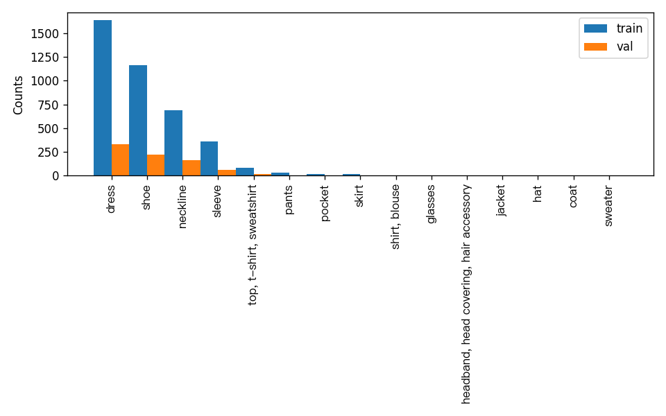
Additionally, the dataset verification also analyzes the distribution of sample numbers across all classes and generates a histogram (histogram.png) for visualization:

Note: Only datasets that pass the verification can be used for training and evaluation.
4.3 Dataset Format Conversion/Dataset Splitting (Optional)
If you need to convert the dataset format or re-split the dataset, you can modify the configuration file or append hyperparameters.
The parameters related to dataset verification can be set by modifying the fields under CheckDataset in the configuration file. Some example explanations for the parameters in the configuration file are as follows:
CheckDataset:convert:enable: Whether to convert the dataset format. Set toTrueto enable dataset format conversion. The default isFalse.src_dataset_type: If dataset format conversion is enabled, you need to set the source dataset format. Available source formats areLabelMeandVOC.
split:enable: Whether to re-split the dataset. Set toTrueto enable dataset splitting. The default isFalse.train_percent: If dataset splitting is enabled, you need to set the percentage of the training set. The value should be an integer between 0 and 100, and the sum withval_percentshould be 100.val_percent: If dataset splitting is enabled, you need to set the percentage of the validation set. The value should be an integer between 0 and 100, and the sum withtrain_percentshould be 100.
Data conversion and data splitting can be enabled simultaneously. The original annotation files for data splitting will be renamed as xxx.bak in the original path. The above parameters can also be set by appending command line arguments, for example, to re-split the dataset and set the training set and validation set ratio: -o CheckDataset.split.enable=True -o CheckDataset.split.train_percent=80 -o CheckDataset.split.val_percent=20.
5. Model Training and Evaluation
5.1 Model Training
Before training, please ensure that you have validated the dataset. To complete PaddleX model training, simply use the following command:
python main.py -c paddlex/configs/object_detection/PicoDet-L.yaml \
    -o Global.mode=train \
    -o Global.dataset_dir=./dataset/det_mini_fashion_pedia_coco \
    -o Train.num_classes=15
PaddleX supports modifying training hyperparameters, single/multi-GPU training, etc., simply by modifying the configuration file or appending command line arguments.
Each model in PaddleX provides a configuration file for model development to set relevant parameters. Model training-related parameters can be set by modifying the Train fields in the configuration file. Some example explanations of parameters in the configuration file are as follows:
Global:mode: Mode, supporting dataset validation (check_dataset), model training (train), and model evaluation (evaluate);device: Training device, options includecpu,gpu,xpu,npu,mlu. For multi-GPU training, specify the card numbers, e.g.,gpu:0,1,2,3;
Train: Training hyperparameter settings;epochs_iters: Number of training epochs;learning_rate: Training learning rate;
For more hyperparameter introductions, please refer to PaddleX General Model Configuration File Parameter Explanation.
Note:
- The above parameters can be set by appending command line arguments, e.g., specifying the mode as model training: -o Global.mode=train; specifying the first two GPUs for training: -o Global.device=gpu:0,1; setting the number of training epochs to 50: -o Train.epochs_iters=50.
- During model training, PaddleX automatically saves model weight files, with the default being output. To specify a save path, use the -o Global.output field in the configuration file.
- PaddleX shields you from the concepts of dynamic graph weights and static graph weights. During model training, both dynamic and static graph weights are produced, and static graph weights are selected by default for model inference.
Training Output Explanation:
After completing model training, all outputs are saved in the specified output directory (default is ./output/), typically including the following:
- train_result.json: Training result record file, recording whether the training task was completed normally, as well as the output weight metrics, relevant file paths, etc.;
- train.log: Training log file, recording model metric changes, loss changes, etc., during training;
- config.yaml: Training configuration file, recording the hyperparameter configuration for this training session;
- .pdparams, .pdema, .pdopt.pdstate, .pdiparams, .pdmodel: Model weight-related files, including network parameters, optimizer, EMA, static graph network parameters, static graph network structure, etc.;
5.2 Model Evaluation
After completing model training, you can evaluate the specified model weight file on the validation set to verify the model accuracy. To evaluate a model using PaddleX, simply use the following command:
python main.py -c paddlex/configs/object_detection/PicoDet-L.yaml \
    -o Global.mode=evaluate \
    -o Global.dataset_dir=./dataset/det_mini_fashion_pedia_coco
Similar to model training, model evaluation supports modifying the configuration file or appending command line arguments.
Note: When evaluating the model, you need to specify the model weight file path. Each configuration file has a built-in default weight save path. If you need to change it, simply set it by appending a command line argument, e.g., -o Evaluate.weight_path=./output/best_model/best_model.pdparams.
5.3 Model Tuning
After learning about model training and evaluation, we can enhance model accuracy by adjusting hyperparameters. By reasonably tuning the number of training epochs, you can control the depth of model training, avoiding overfitting or underfitting. Meanwhile, the setting of the learning rate is crucial to the speed and stability of model convergence. Therefore, when optimizing model performance, it is essential to carefully consider the values of these two parameters and adjust them flexibly based on actual conditions to achieve the best training results.
It is recommended to follow the controlled variable method when debugging parameters:
- First, fix the number of training epochs at 50 and the batch size at 16.
- Initiate three experiments based on the PicoDet-L model with learning rates of: 0.02, 0.04, 0.08.
- It can be observed that the configuration with the highest accuracy in Experiment 2 is a learning rate of 0.04. Based on this training hyperparameter, change the number of epochs and observe the accuracy results at different epochs, finding that the best accuracy is generally achieved at 80 epochs.
Learning Rate Exploration Results:
| Experiment | Epochs | Learning Rate | batch_size | Training Environment | mAP@0.5 |
|---|---|---|---|---|---|
| Experiment 1 | 50 | 0.02 | 16 | 4 GPUs | 0.428 |
| Experiment 2 | 50 | 0.04 | 16 | 4 GPUs | 0.471 |
| Experiment 3 | 50 | 0.08 | 16 | 4 GPUs | 0.440 |
Epoch Variation Results:
| Experiment | Epochs | Learning Rate | batch_size | Training Environment | mAP@0.5 |
|---|---|---|---|---|---|
| Experiment 2 | 50 | 0.04 | 16 | 4 GPUs | 0.471 |
| Reduced Epochs in Exp. 2 | 30 | 0.04 | 16 | 4 GPUs | 0.425 |
| Increased Epochs in Exp. 2 | 80 | 0.04 | 16 | 4 GPUs | 0.491 |
| Further Increased Epochs | 100 | 0.04 | 16 | 4 GPUs | 0.459 |
Note: This tutorial is designed for a 4-GPU setup. If you have only 1 GPU, you can adjust the number of training GPUs to complete the experiments, but the final metrics may not align with the above figures, which is normal.
6. Pipeline Testing
Replace the model in the pipeline with the fine-tuned model for testing, e.g.:
python main.py -c paddlex/configs/object_detection/PicoDet-L.yaml \
    -o Global.mode=predict \
    -o Predict.model_dir="output/best_model/inference" \
    -o Predict.input="https://paddle-model-ecology.bj.bcebos.com/paddlex/PaddleX3.0/application/object_detection/FashionPedia_demo.png"
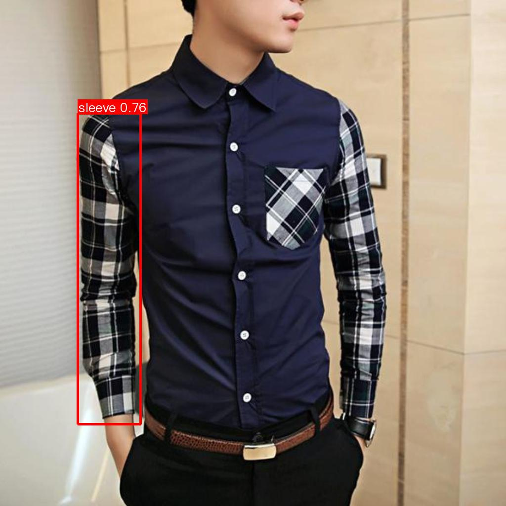
The prediction results will be generated under ./output, and the prediction result for FashionPedia_demo.png is as follows:

7. Development Integration/Deployment
If the General Object Detection Pipeline meets your requirements for inference speed and precision in your production line, you can proceed directly with development integration/deployment.
- Directly apply the trained model in your Python project by referring to the following sample code, and modify the
Pipeline.modelin thepaddlex/pipelines/object_detection.yamlconfiguration file to your own model path:
from paddlex import create_pipeline
pipeline = create_pipeline(pipeline="paddlex/pipelines/object_detection.yaml")
output = pipeline.predict("https://paddle-model-ecology.bj.bcebos.com/paddlex/PaddleX3.0/application/object_detection/FashionPedia_demo.png")
for res in output:
    res.print() # Print the structured output of the prediction
    res.save_to_img("./output/") # Save the visualized result image
    res.save_to_json("./output/") # Save the structured output of the prediction
For more parameters, please refer to General Object Detection Pipeline Usage Tutorial.
-
Additionally, PaddleX offers three other deployment methods, detailed as follows:
-
high-performance inference: In actual production environments, many applications have stringent standards for deployment strategy performance metrics (especially response speed) to ensure efficient system operation and smooth user experience. To this end, PaddleX provides high-performance inference plugins aimed at deeply optimizing model inference and pre/post-processing for significant end-to-end process acceleration. For detailed high-performance inference procedures, please refer to the PaddleX High-Performance Inference Guide.
- Service-Oriented Deployment: Service-oriented deployment is a common deployment form in actual production environments. By encapsulating inference functions as services, clients can access these services through network requests to obtain inference results. PaddleX supports users in achieving cost-effective service-oriented deployment of production lines. For detailed service-oriented deployment procedures, please refer to the PaddleX Service-Oriented Deployment Guide.
- Edge Deployment: Edge deployment is a method that places computing and data processing capabilities directly on user devices, allowing devices to process data without relying on remote servers. PaddleX supports deploying models on edge devices such as Android. For detailed edge deployment procedures, please refer to the PaddleX Edge Deployment Guide.
You can select the appropriate deployment method for your model pipeline according to your needs, and proceed with subsequent AI application integration.