PaddleX 3.0 Document Scene Information Extraction v3 (PP-ChatOCRv3_doc) —— Tutorial on Paper and Literature Information Extraction
PaddleX offers a rich set of pipelines, each consisting of one or more models that can tackle specific scenario tasks. All PaddleX pipelines support quick trials, and if the results are not satisfactory, you can fine-tune the models with your private data. PaddleX also provides Python APIs for easy integration into personal projects. Before use, you need to install PaddleX. For installation instructions, please refer to PaddleX Installation. This tutorial introduces the usage of the pipeline tool with a garbage classification task as an example.
1. Select a Pipeline
Document information extraction is a part of document processing with widespread applications in numerous scenarios, such as academic research, library management, scientific and technological intelligence analysis, and literature review writing. Through document information extraction technology, we can automatically extract key information from academic papers, including titles, authors, abstracts, keywords, publication years, journal names, citation information, and more, and store this information in a structured format for easy subsequent retrieval, analysis, and application. This not only enhances the work efficiency of researchers but also provides strong support for the in-depth development of academic research.
Firstly, it is necessary to select the corresponding PaddleX pipeline based on the task scenario. This section takes information extraction from academic papers as an example to introduce how to conduct secondary development for tasks related to the Document Scene Information Extraction v3 pipeline, which corresponds to the Document Scene Information Extraction v3 in PaddleX. If you are unsure about the correspondence between tasks and pipelines, you can refer to the capability introductions of related pipelines in the PaddleX Supported Pipelines List.
2. Quick Start
PaddleX offers two ways to experience its capabilities. You can try out the Document Scene Information Extraction v3 pipeline online, or you can use Python locally to experience the effects of the Document Scene Information Extraction v3 pipeline.
2.1 Local Experience
Before using the Document Scene Information Extraction v3 pipeline locally, please ensure that you have completed the installation of the PaddleX wheel package according to the PaddleX Local Installation Tutorial. With just a few lines of code, you can quickly perform inference using the pipeline:
from paddlex import create_pipeline

pipeline = create_pipeline(
    pipeline="PP-ChatOCRv3-doc",
    llm_name="ernie-3.5",
    llm_params={"api_type": "qianfan", "ak": "", "sk": ""} # To use the Qianfan API, please fill in your Access Key (ak) and Secret Key (sk), as you will not be able to invoke large models without them.
    # llm_params={"api_type": "aistudio", "access_token": ""} # Or, to use the AIStudio API, please fill in your access_token, as you will not be able to invoke large models without it.
    )

visual_result, visual_info = pipeline.visual_predict("https://paddle-model-ecology.bj.bcebos.com/paddlex/PaddleX3.0/doc_images/practical_tutorial/PP-ChatOCRv3_doc_layout/test.jpg")

for res in visual_result:
    res.save_to_img("./output")
    res.save_to_html('./output')
    res.save_to_xlsx('./output')

vector = pipeline.build_vector(visual_info=visual_info)
chat_result = pipeline.chat(
    key_list=["header", "table caption"],
    visual_info=visual_info,
    vector=vector,
    )
chat_result.print()
Note: Currently, the large language model only supports Ernie. You can obtain the relevant ak/sk (access_token) on the Baidu Cloud Qianfan Platform or Baidu AIStudio Community. If you use the Baidu Cloud Qianfan Platform, you can refer to the AK and SK Authentication API Calling Process to obtain ak/sk. If you use Baidu AIStudio Community, you can obtain the access_token from the Baidu AIStudio Community Access Token.
The printed output results are as follows:
The result has been saved in output/tmpfnss9sq9_layout.jpg.
The result has been saved in output/tmpfnss9sq9_ocr.jpg.
The result has been saved in output/tmpfnss9sq9_table.jpg.
The result has been saved in output/tmpfnss9sq9_table.jpg.
The result has been saved in output/tmpfnss9sq9/tmpfnss9sq9.html.
The result has been saved in output/tmpfnss9sq9/tmpfnss9sq9.html.
The result has been saved in output/tmpfnss9sq9/tmpfnss9sq9.xlsx.
The result has been saved in output/tmpfnss9sq9/tmpfnss9sq9.xlsx.

{'chat_res': {'页眉': '未知', '图表标题': '未知'}, 'prompt': ''}
In the output directory, the visualization results of layout area detection, OCR, table recognition, as well as the table results in HTML and XLSX formats, are saved.
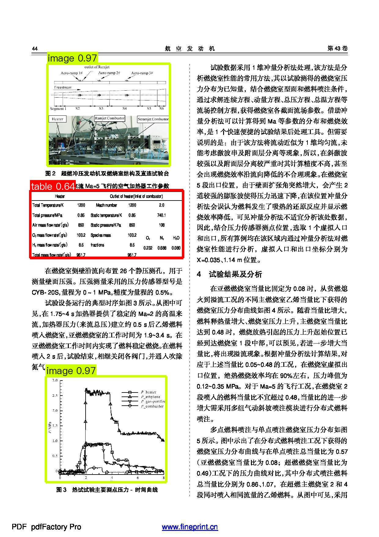
Among them, the visualization of the layout area detection results is as follows:

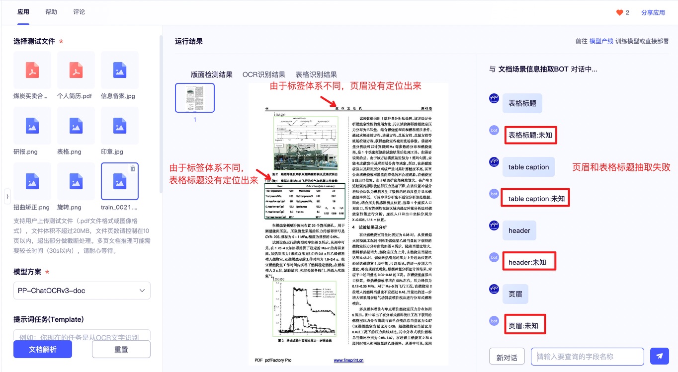
Through the online experience of the document scene information extraction, a Badcase analysis can be conducted to identify issues with the official model of the document scene information extraction pipeline. Due to the current limitation of the official model, which only distinguishes among figures, tables, and seals, it is currently unable to accurately locate and extract other information such as headers and table titles. The results for these in {'chat_res': {'header': 'unknown', 'table caption': 'unknown'}, 'prompt': ''} are unknown. Therefore, this section focuses on the scenario of academic papers. Utilizing a dataset of academic paper documents, with the extraction of header and chart title information as examples, the layout analysis model within the document scene information extraction pipeline is fine-tuned to achieve the ability to accurately extract header and table title information from the document.
2.2 Online Experience
You can experience the effectiveness of the Document Scene Information Extraction v3 pipeline on the AIStudio Community. Click the link to download the Test Paper Document File, and then upload it to the official Document Scene Information Extraction v3 application to experience the extraction results. The process is as follows:

3. Choosing a Model
PaddleX provides 4 end-to-end layout detection models, which can be referenced in the Model List. Some of the benchmarks for these models are as follows:
| Model | mAP(0.5) (%) | GPU Inference Time (ms) | CPU Inference Time (ms) | Model Size (M) | Description |
|---|---|---|---|---|---|
| PicoDet_layout_1x | 86.8 | 13.0 | 91.3 | 7.4 | An efficient layout area localization model trained on the PubLayNet dataset based on PicoDet-1x can locate five types of areas, including text, titles, tables, images, and lists. |
| PicoDet_layout_1x_table | 95.7 | 12.623 | 90.8934 | 7.4 M | An efficient layout area localization model trained on the PubLayNet dataset based on PicoDet-1x can locate one type of tables. |
| PicoDet-S_layout_3cls | 87.1 | 13.5 | 45.8 | 4.8 | An high-efficient layout area localization model trained on a self-constructed dataset based on PicoDet-S for scenarios such as Chinese and English papers, magazines, and research reports includes three categories: tables, images, and seals. |
| PicoDet-S_layout_17cls | 70.3 | 13.6 | 46.2 | 4.8 | A high-efficient layout area localization model trained on a self-constructed dataset based on PicoDet-S_layout_17cls for scenarios such as Chinese and English papers, magazines, and research reports includes 17 common layout categories, namely: paragraph titles, images, text, numbers, abstracts, content, chart titles, formulas, tables, table titles, references, document titles, footnotes, headers, algorithms, footers, and seals. |
| PicoDet-L_layout_3cls | 89.3 | 15.7 | 159.8 | 22.6 | An efficient layout area localization model trained on a self-constructed dataset based on PicoDet-L for scenarios such as Chinese and English papers, magazines, and research reports includes three categories: tables, images, and seals. |
| PicoDet-L_layout_17cls | 79.9 | 17.2 | 160.2 | 22.6 | A efficient layout area localization model trained on a self-constructed dataset based on PicoDet-L_layout_17cls for scenarios such as Chinese and English papers, magazines, and research reports includes 17 common layout categories, namely: paragraph titles, images, text, numbers, abstracts, content, chart titles, formulas, tables, table titles, references, document titles, footnotes, headers, algorithms, footers, and seals. |
| RT-DETR-H_layout_3cls | 95.9 | 114.6 | 3832.6 | 470.1 | A high-precision layout area localization model trained on a self-constructed dataset based on RT-DETR-H for scenarios such as Chinese and English papers, magazines, and research reports includes three categories: tables, images, and seals. |
| RT-DETR-H_layout_17cls | 92.6 | 115.1 | 3827.2 | 470.2 | A high-precision layout area localization model trained on a self-constructed dataset based on RT-DETR-H for scenarios such as Chinese and English papers, magazines, and research reports includes 17 common layout categories, namely: paragraph titles, images, text, numbers, abstracts, content, chart titles, formulas, tables, table titles, references, document titles, footnotes, headers, algorithms, footers, and seals. |
Note: The evaluation set for the above accuracy metrics is PaddleOCR's self-built layout region analysis dataset, containing 10,000 images of common document types, including English and Chinese papers, magazines, research reports, etc. GPU inference time is based on an NVIDIA Tesla T4 machine with FP32 precision. CPU inference speed is based on an Intel(R) Xeon(R) Gold 5117 CPU @ 2.00GHz with 8 threads and FP32 precision.
4. Data Preparation and Verification
4.1 Data Preparation
This tutorial uses the Academic paper literature Dataset as an example dataset. You can obtain the example dataset using the following commands. If you are using your own annotated dataset, you need to adjust it according to PaddleX's format requirements to meet PaddleX's data format specifications. For an introduction to data formats, you can refer to the PaddleX Object Detection Task Module Data Annotation Tutorial.
Dataset acquisition commands:
cd /path/to/paddlex
wget https://paddle-model-ecology.bj.bcebos.com/paddlex/data/paperlayout.tar -P ./dataset
tar -xf ./dataset/paperlayout.tar -C ./dataset/
4.2 Dataset Verification
To verify the dataset, simply run the following command:
python main.py -c paddlex/configs/layout_detection/RT-DETR-H_layout_3cls.yaml \
    -o Global.mode=check_dataset \
    -o Global.dataset_dir=./dataset/paperlayout/
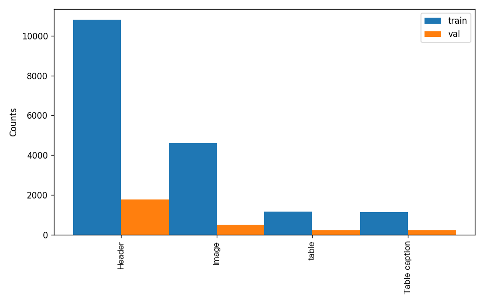
After executing the above command, PaddleX will verify the dataset and count the basic information of the dataset. If the command runs successfully, it will print Check dataset passed ! in the log, and the relevant outputs will be saved in the current directory's ./output/check_dataset directory. The output directory includes visualized example images and a histogram of sample distribution. The verification result file is saved in ./output/check_dataset_result.json, and the specific content of the verification result file is as follows:
{
  "done_flag": true,
  "check_pass": true,
  "attributes": {
    "num_classes": 4,
    "train_samples": 4734,
    "train_sample_paths": [
      "check_dataset\/demo_img\/train_4612.jpg",
      "check_dataset\/demo_img\/train_4844.jpg",
      "check_dataset\/demo_img\/train_0084.jpg",
      "check_dataset\/demo_img\/train_0448.jpg",
      "check_dataset\/demo_img\/train_4703.jpg",
      "check_dataset\/demo_img\/train_3572.jpg",
      "check_dataset\/demo_img\/train_4516.jpg",
      "check_dataset\/demo_img\/train_2836.jpg",
      "check_dataset\/demo_img\/train_1353.jpg",
      "check_dataset\/demo_img\/train_0225.jpg"
    ],
    "val_samples": 928,
    "val_sample_paths": [
      "check_dataset\/demo_img\/val_0982.jpg",
      "check_dataset\/demo_img\/val_0607.jpg",
      "check_dataset\/demo_img\/val_0623.jpg",
      "check_dataset\/demo_img\/val_0890.jpg",
      "check_dataset\/demo_img\/val_0036.jpg",
      "check_dataset\/demo_img\/val_0654.jpg",
      "check_dataset\/demo_img\/val_0895.jpg",
      "check_dataset\/demo_img\/val_0059.jpg",
      "check_dataset\/demo_img\/val_0142.jpg",
      "check_dataset\/demo_img\/val_0088.jpg"
    ]
  },
  "analysis": {
    "histogram": "check_dataset\/histogram.png"
  },
  "dataset_path": ".\/dataset\/paperlayout\/",
  "show_type": "image",
  "dataset_type": "COCODetDataset"
}
In the above verification results, check_pass being True indicates that the dataset format meets the requirements. Explanations for other indicators are as follows:
attributes.num_classes: The number of classes in this dataset is 4, which is the number of classes that need to be passed in for subsequent training;attributes.train_samples: The number of training set samples in this dataset is 4734;attributes.val_samples: The number of validation set samples in this dataset is 928;attributes.train_sample_paths: A list of relative paths to the visualized images of the training set samples in this dataset;attributes.val_sample_paths: A list of relative paths to the visualized images of the validation set samples in this dataset;
In addition, the dataset verification also analyzes the sample number distribution of all categories in the dataset and draws a distribution histogram (histogram.png):

Note: Only data that passes the verification can be used for training and evaluation.
4.3 Dataset Splitting (Optional)
If you need to convert the dataset format or re-split the dataset, you can set it by modifying the configuration file or appending hyperparameters.
The parameters related to dataset verification can be set by modifying the fields under CheckDataset in the configuration file. Some example explanations of the parameters in the configuration file are as follows:
CheckDataset:split:enable: Whether to re-split the dataset. When set toTrue, the dataset format will be converted. The default isFalse;train_percent: If the dataset is to be re-split, you need to set the percentage of the training set. The type is any integer between 0-100, and it needs to ensure that the sum withval_percentis 100;val_percent: If the dataset is to be re-split, you need to set the percentage of the validation set. The type is any integer between 0-100, and it needs to ensure that the sum withtrain_percentis 100;
Data Splitting
When splitting data, the original annotation files will be renamed as xxx.bak in the original path. The above parameters can also be set by appending command line arguments, for example, to re-split the dataset and set the ratio of training set to validation set: -o CheckDataset.split.enable=True -o CheckDataset.split.train_percent=80 -o CheckDataset.split.val_percent=20.
5. Model Training and Evaluation
5.1 Model Training
Before training, please ensure that you have validated the dataset. To complete PaddleX model training, simply use the following command:
python main.py -c paddlex/configs/layout_detection/RT-DETR-H_layout_3cls.yaml \
    -o Global.mode=train \
    -o Global.dataset_dir=./dataset/paperlayout \
    -o Train.num_classes=4
PaddleX supports modifying training hyperparameters, single/multi-GPU training, etc., by modifying the configuration file or appending command line arguments.
Each model in PaddleX provides a configuration file for model development to set relevant parameters. Model training-related parameters can be set by modifying the Train fields in the configuration file. Some example explanations of parameters in the configuration file are as follows:
Global:mode: Mode, supporting dataset validation (check_dataset), model training (train), and model evaluation (evaluate);device: Training device, options includecpu,gpu,xpu,npu,mlu. For multi-GPU training, specify the card numbers, e.g.,gpu:0,1,2,3;
Train: Training hyperparameter settings;epochs_iters: Number of training epochs;learning_rate: Training learning rate;
For more hyperparameter introductions, please refer to PaddleX General Model Configuration File Parameter Explanation.
Note:
- The above parameters can be set by appending command line arguments, e.g., specifying the mode as model training: -o Global.mode=train; specifying the first two GPUs for training: -o Global.device=gpu:0,1; setting the number of training epochs to 10: -o Train.epochs_iters=10.
- During model training, PaddleX automatically saves model weight files, with the default being output. If you need to specify a save path, you can use the -o Global.output field in the configuration file.
- PaddleX shields you from the concepts of dynamic graph weights and static graph weights. During model training, both dynamic and static graph weights are produced, and static graph weights are selected by default for model inference.
Explanation of Training Outputs:
After completing model training, all outputs are saved in the specified output directory (default is ./output/), typically including the following:
- train_result.json: Training result record file, recording whether the training task was completed normally, as well as the output weight metrics and related file paths;
- train.log: Training log file, recording changes in model metrics and loss during training;
- config.yaml: Training configuration file, recording the hyperparameter configuration for this training session;
- .pdparams, .pdopt, .pdstates, .pdiparams, .pdmodel: Model weight-related files, including network parameters, optimizer, static graph network parameters, static graph network structure, etc.;
5.2 Model Evaluation
After completing model training, you can evaluate the specified model weight file on the validation set to verify the model accuracy. To evaluate a model using PaddleX, simply use the following command:
python main.py -c paddlex/configs/layout_detection/RT-DETR-H_layout_3cls.yaml \
    -o Global.mode=evaluate \
    -o Global.dataset_dir=./dataset/paperlayout
Similar to model training, model evaluation supports setting by modifying the configuration file or appending command line arguments.
Note: When evaluating the model, you need to specify the model weight file path. Each configuration file has a default weight save path. If you need to change it, simply set it by appending a command line argument, e.g., -o Evaluate.weight_path=./output/best_model/best_model.pdparams.
5.3 Model Optimization
After learning about model training and evaluation, we can enhance model accuracy by adjusting hyperparameters. By carefully tuning the number of training epochs, you can control the depth of model training to avoid overfitting or underfitting. Meanwhile, the setting of the learning rate is crucial to the speed and stability of model convergence. Therefore, when optimizing model performance, it is essential to consider the values of these two parameters prudently and adjust them flexibly based on actual conditions to achieve the best training results.
It is recommended to follow the controlled variable method when debugging parameters:
- First, fix the number of training epochs at 30, and set the batch size to 4 due to the small size of the training dataset.
- Initiate four experiments based on the
RT-DETR-H_layout_3clsmodel, with learning rates of: 0.001,0.0005,0.0001,0.00001. - It can be observed that the configuration with the highest accuracy in Experiment 2 is a learning rate of 0.0001. Based on this training hyperparameter, change the number of epochs and observe the accuracy results at different epochs, finding that the best accuracy is generally achieved at 50 and 100 epochs.
Learning Rate Exploration Results:
| Experiment ID | Learning Rate | mAP@@0.50:0.95 |
|---|---|---|
| 1 | 0.00001 | 88.90 |
| 2 | 0.0001 | 92.41 |
| 3 | 0.0005 | 92.27 |
| 4 | 0.001 | 90.66 |
Next, we can increase the number of training epochs based on a learning rate set to 0.001. Comparing experiments [2, 4, 5] below, it can be seen that as the number of training epochs increases, the model's accuracy further improves.
| Experiment ID | Learning Rate | mAP@@0.50:0.95 |
|---|---|---|
| 2 | 30 | 92.41 |
| 4 | 50 | 92.63 |
| 5 | 100 | 92.88 |
Note: This tutorial is designed for a 4-GPU setup. If you only have 1 GPU, you can complete the experiment by adjusting the number of training GPUs, but the final metrics may not align perfectly with the above indicators, which is normal.
When selecting a training environment, it is important to consider the relationship between the number of training GPUs, the total batch_size, and the learning rate. Firstly, the total batch_size is equal to the number of training GPUs multiplied by the batch_size per GPU. Secondly, the total batch_size and the learning rate are related, and the learning rate should be adjusted in synchronization with the total batch_size. The default learning rate corresponds to a total batch_size based on 4 GPUs. If you plan to train in a single-GPU environment, you need to divide the learning rate by 4 accordingly. If you plan to train in an 8-GPU environment, you need to multiply the learning rate by 2 accordingly.
For reference, the command to execute training with different parameter adjustments can be:
python main.py -c paddlex/configs/layout_detection/RT-DETR-H_layout_3cls.yaml \
    -o Global.mode=train \
    -o Global.dataset_dir=./dataset/paperlayout \
    -o Train.num_classes=4 \
    -o Train.learning_rate=0.0001 \
    -o Train.epochs_iters=30 \
    -o Train.batch_size=4
5.4 Model Inference
You can test the fine-tuned single model using test file
python main.py -c paddlex/configs/layout_detection/RT-DETR-H_layout_3cls.yaml \
    -o Global.mode=predict \
    -o Predict.model_dir="output/best_model/inference" \
    -o Predict.input="https://paddle-model-ecology.bj.bcebos.com/paddlex/PaddleX3.0/doc_images/practical_tutorial/PP-ChatOCRv3_doc_layout/test.jpg"
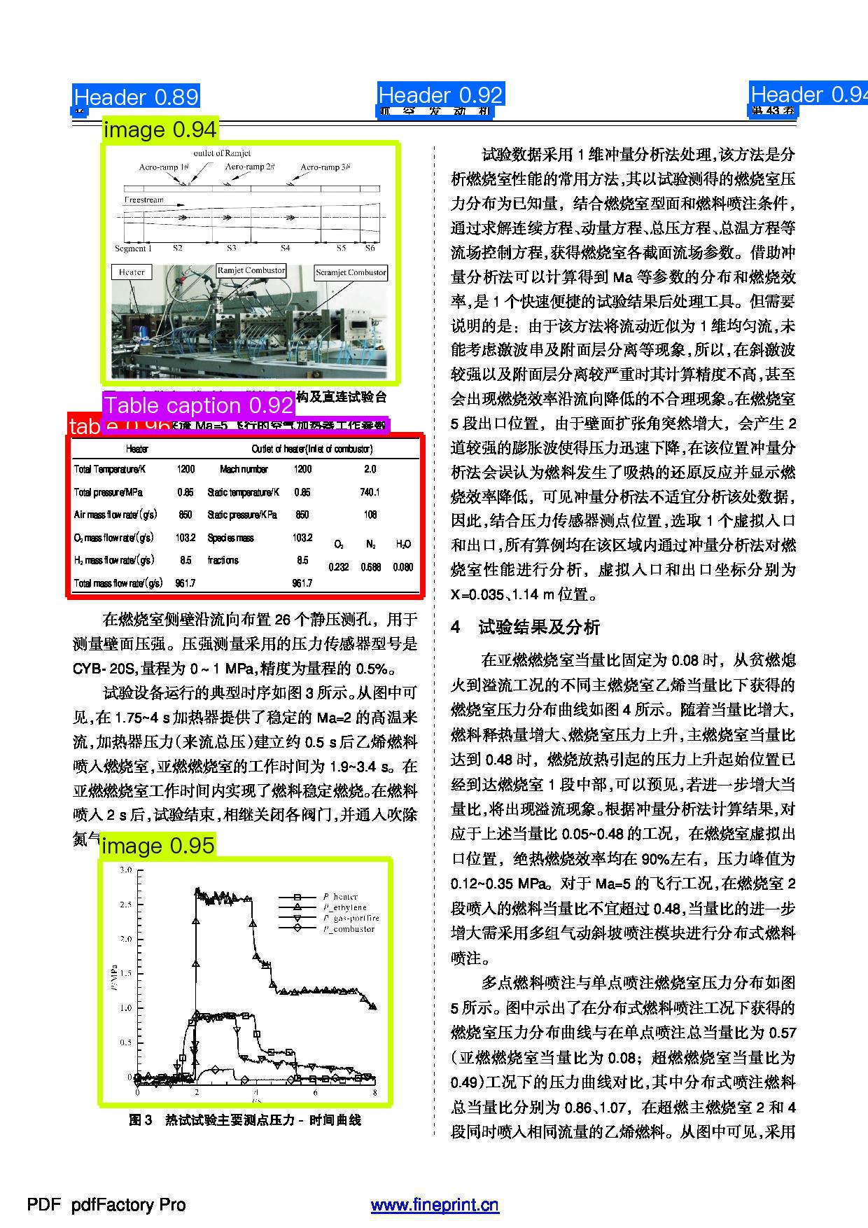
By following the above steps, prediction results can be generated under the ./output directory. The layout prediction result for test.jpg is as follows:

6. Pipeline Inference
Replace the model in the production line with the fine-tuned model for testing, and use the academic paper literature test file to perform predictions.
First, obtain and update the configuration file for the Document Information Extraction v3. Execute the following command to retrieve the configuration file (assuming a custom save location of ./my_path):
Modify the Pipeline.layout_model field in PP-ChatOCRv3-doc.yaml to the path of the fine-tuned model mentioned above. The modified configuration is as follows:
Pipeline:
  layout_model: ./output/best_model/inference
  table_model: SLANet_plus
  text_det_model: PP-OCRv4_server_det
  text_rec_model: PP-OCRv4_server_rec
  seal_text_det_model: PP-OCRv4_server_seal_det
  doc_image_ori_cls_model: null
  doc_image_unwarp_model: null
  llm_name: "ernie-3.5"
  llm_params:
    api_type: qianfan
    ak:
    sk:
After making the modifications, you only need to change the value of the pipeline parameter in the create_pipeline method to the path of the production line configuration file to apply the configuration.
from paddlex import create_pipeline

pipeline = create_pipeline(
    pipeline="./my_path/PP-ChatOCRv3-doc.yaml",
    llm_name="ernie-3.5",
    llm_params={"api_type": "qianfan", "ak": "", "sk": ""} # To use the Qianfan API, please fill in your Access Key (ak) and Secret Key (sk), as you will not be able to invoke large models without them.
    # llm_params={"api_type": "aistudio", "access_token": ""} # Or, to use the AIStudio API, please fill in your access_token, as you will not be able to invoke large models without it.
    )

visual_result, visual_info = pipeline.visual_predict("https://paddle-model-ecology.bj.bcebos.com/paddlex/PaddleX3.0/doc_images/practical_tutorial/PP-ChatOCRv3_doc_layout/test.jpg")

for res in visual_result:
    res.save_to_img("./output_ft")
    res.save_to_html('./output_ft')
    res.save_to_xlsx('./output_ft')

vector = pipeline.build_vector(visual_info=visual_info)
chat_result = pipeline.chat(
    key_list=["header", "table caption"],
    visual_info=visual_info,
    vector=vector,
    )
chat_result.print()
By following the above steps, prediction results can be generated under ./output_ft, and the printed key information extraction results are as follows:
{'chat_res': {'header': '第43卷\n 航空发动机\n 44', 'table caption': '表1模拟来流Ma=5飞行的空气加热器工作参数'}, 'prompt': ''}
It can be observed that after fine-tuning the model, the key information has been correctly extracted.
The visualization result of the layout is as follows, with the correctly added ability to locate the areas of headers and table titles:

7. Development Integration/Deployment
If the Document Scene Information Extraction v3 production line meets your requirements for inference speed and accuracy, you can proceed directly with development integration/deployment.
- Directly apply the trained model production line in your Python project, as shown in the following code:
from paddlex import create_pipeline

pipeline = create_pipeline(
    pipeline="./my_path/PP-ChatOCRv3-doc.yaml",
    llm_name="ernie-3.5",
    llm_params={"api_type": "qianfan", "ak": "", "sk": ""} # To use the Qianfan API, please fill in your Access Key (ak) and Secret Key (sk), as you will not be able to invoke large models without them.
    # llm_params={"api_type": "aistudio", "access_token": ""} # Or, to use the AIStudio API, please fill in your access_token, as you will not be able to invoke large models without it.
    )

visual_result, visual_info = pipeline.visual_predict("https://paddle-model-ecology.bj.bcebos.com/paddlex/PaddleX3.0/doc_images/practical_tutorial/PP-ChatOCRv3_doc_layout/test.jpg")

for res in visual_result:
    res.save_to_img("./output")
    res.save_to_html('./output')
    res.save_to_xlsx('./output')

vector = pipeline.build_vector(visual_info=visual_info)
chat_result = pipeline.chat(
    key_list=["header", "table caption"],
    visual_info=visual_info,
    vector=vector,
    )
chat_result.print()
For more parameters, please refer to the Document Scene Information Extraction Pipeline Usage Tutorial.
-
Additionally, PaddleX offers three other deployment methods, detailed as follows:
-
high-performance inference: In actual production environments, many applications have stringent standards for deployment strategy performance metrics (especially response speed) to ensure efficient system operation and smooth user experience. To this end, PaddleX provides high-performance inference plugin aimed at deeply optimizing model inference and pre/post-processing for significant end-to-end process acceleration. For detailed high-performance inference procedures, please refer to the PaddleX High-Performance Inference Guide.
- Service-Oriented Deployment: Service-oriented deployment is a common deployment form in actual production environments. By encapsulating inference functions as services, clients can access these services through network requests to obtain inference results. PaddleX supports users in achieving cost-effective service-oriented deployment of production lines. For detailed service-oriented deployment procedures, please refer to the PaddleX Service-Oriented Deployment Guide.
- Edge Deployment: Edge deployment is a method that places computing and data processing capabilities directly on user devices, allowing devices to process data without relying on remote servers. PaddleX supports deploying models on edge devices such as Android. For detailed edge deployment procedures, please refer to the PaddleX Edge Deployment Guide.
You can select the appropriate deployment method for your model pipeline according to your needs, and proceed with subsequent AI application integration.