公式识别产线使用教程
1. 公式识别产线介绍
公式识别是一种自动从文档或图像中识别和提取LaTeX公式内容及其结构的技术,广泛应用于数学、物理、计算机科学等领域的文档编辑和数据分析。通过使用计算机视觉和机器学习算法,公式识别能够将复杂的数学公式信息转换为可编辑的LaTeX格式,方便用户进一步处理和分析数据。
公式识别产线用于解决公式识别任务,提取图片中的公式信息以LaTeX源码形式输出,本产线是一个集成了百度飞桨视觉团队自研的先进公式识别模型PP-FormulaNet 和业界知名公式识别模型 UniMERNet的端到端公式识别系统,支持简单印刷公式、复杂印刷公式、手写公式的识别,并在此基础上,增加了对图像的方向矫正和扭曲矫正功能。基于本产线,可实现公式内容精准预测,使用场景覆盖教育、科研、金融、制造等各个领域。本产线同时提供了灵活的服务化部署方式,支持在多种硬件上使用多种编程语言调用。不仅如此,本产线也提供了二次开发的能力,您可以基于本产线在您自己的数据集上训练调优,训练后的模型也可以无缝集成。

公式识别产线中包含以下4个模块。每个模块均可独立进行训练和推理,并包含多个模型。有关详细信息,请点击相应模块以查看文档。
- 公式识别模块
- 版面区域检测模块(可选)
- 文档图像方向分类模块 (可选)
- 文本图像矫正模块 (可选)
在本产线中,您可以根据下方的基准测试数据选择使用的模型。
文档图像方向分类模块(可选):
| 模型 | 模型下载链接 | Top-1 Acc(%) | GPU推理耗时(ms) [常规模式 / 高性能模式] |
CPU推理耗时(ms) [常规模式 / 高性能模式] |
模型存储大小(MB) | 介绍 |
|---|---|---|---|---|---|---|
| PP-LCNet_x1_0_doc_ori | 推理模型/训练模型 | 99.06 | 2.62 / 0.59 | 3.24 / 1.19 | 7 | 基于PP-LCNet_x1_0的文档图像分类模型,含有四个类别,即0度,90度,180度,270度 |
文本图像矫正模块(可选):
| 模型 | 模型下载链接 | CER | GPU推理耗时(ms) [常规模式 / 高性能模式] |
CPU推理耗时(ms) [常规模式 / 高性能模式] |
模型存储大小(MB) | 介绍 |
|---|---|---|---|---|---|---|
| UVDoc | 推理模型/训练模型 | 0.179 | 19.05 / 19.05 | - / 869.82 | 30.3 | 高精度文本图像矫正模型 |
版面区域检测模块(可选):
* 版面检测模型,包含20个常见的类别:文档标题、段落标题、文本、页码、摘要、目录、参考文献、脚注、页眉、页脚、算法、公式、公式编号、图像、表格、图和表标题(图标题、表格标题和图表标题)、印章、图表、侧栏文本和参考文献内容| 模型 | 模型下载链接 | mAP(0.5)(%) | GPU推理耗时(ms) [常规模式 / 高性能模式] |
CPU推理耗时(ms) [常规模式 / 高性能模式] |
模型存储大小(MB) | 介绍 |
|---|---|---|---|---|---|---|
| PP-DocLayout_plus-L | 推理模型/训练模型 | 83.2 | 53.03 / 17.23 | 634.62 / 378.32 | 126.01 | 基于RT-DETR-L在包含中英文论文、多栏杂志、报纸、PPT、合同、书本、试卷、研报、古籍、日文文档、竖版文字文档等场景的自建数据集训练的更高精度版面区域定位模型 |
| 模型 | 模型下载链接 | mAP(0.5)(%) | GPU推理耗时(ms) [常规模式 / 高性能模式] |
CPU推理耗时(ms) [常规模式 / 高性能模式] |
模型存储大小(MB) | 介绍 |
|---|---|---|---|---|---|---|
| PP-DocLayout-L | 推理模型/训练模型 | 90.4 | 33.59 / 33.59 | 503.01 / 251.08 | 123.76 | 基于RT-DETR-L在包含中英文论文、杂志、合同、书本、试卷和研报等场景的自建数据集训练的高精度版面区域定位模型 |
| PP-DocLayout-M | 推理模型/训练模型 | 75.2 | 13.03 / 4.72 | 43.39 / 24.44 | 22.578 | 基于PicoDet-L在包含中英文论文、杂志、合同、书本、试卷和研报等场景的自建数据集训练的精度效率平衡的版面区域定位模型 |
| PP-DocLayout-S | 推理模型/训练模型 | 70.9 | 11.54 / 3.86 | 18.53 / 6.29 | 4.834 | 基于PicoDet-S在中英文论文、杂志、合同、书本、试卷和研报等场景上自建数据集训练的高效率版面区域定位模型 |
👉模型列表详情
* 版面区域检测模型,包含17个版面常见类别,分别是:段落标题、图片、文本、数字、摘要、内容、图表标题、公式、表格、表格标题、参考文献、文档标题、脚注、页眉、算法、页脚、印章| 模型 | 模型下载链接 | mAP(0.5)(%) | GPU推理耗时(ms) | CPU推理耗时 (ms) | 模型存储大小(MB) | 介绍 |
|---|---|---|---|---|---|---|
| PicoDet-S_layout_17cls | 推理模型/训练模型 | 87.4 | 8.80 / 3.62 | 17.51 / 6.35 | 4.8 | 基于PicoDet-S轻量模型在中英文论文、杂志和研报等场景上自建数据集训练的高效率版面区域定位模型 |
| PicoDet-L_layout_17cls | 推理模型/训练模型 | 89.0 | 12.60 / 10.27 | 43.70 / 24.42 | 22.6 | 基于PicoDet-L在中英文论文、杂志和研报等场景上自建数据集训练的效率精度均衡版面区域定位模型 |
| RT-DETR-H_layout_17cls | 推理模型/训练模型 | 98.3 | 115.29 / 101.18 | 964.75 / 964.75 | 470.2 | 基于RT-DETR-H在中英文论文、杂志和研报等场景上自建数据集训练的高精度版面区域定位模型 |
| 模型 | 模型下载链接 | mAP(0.5)(%) | GPU推理耗时(ms) [常规模式 / 高性能模式] |
CPU推理耗时(ms) [常规模式 / 高性能模式] |
模型存储大小(MB) | 介绍 |
|---|---|---|---|---|---|---|
| PP-DocLayout-L | 推理模型/训练模型 | 90.4 | 33.59 / 33.59 | 503.01 / 251.08 | 123.76 | 基于RT-DETR-L在包含中英文论文、杂志、合同、书本、试卷和研报等场景的自建数据集训练的高精度版面区域定位模型 |
| PP-DocLayout-M | 推理模型/训练模型 | 75.2 | 13.03 / 4.72 | 43.39 / 24.44 | 22.578 | 基于PicoDet-L在包含中英文论文、杂志、合同、书本、试卷和研报等场景的自建数据集训练的精度效率平衡的版面区域定位模型 |
| PP-DocLayout-S | 推理模型/训练模型 | 70.9 | 11.54 / 3.86 | 18.53 / 6.29 | 4.834 | 基于PicoDet-S在中英文论文、杂志、合同、书本、试卷和研报等场景上自建数据集训练的高效率版面区域定位模型 |
| 模型 | 模型下载链接 | mAP(0.5)(%) | GPU推理耗时(ms) [常规模式 / 高性能模式] |
CPU推理耗时(ms) [常规模式 / 高性能模式] |
模型存储大小(MB) | 介绍 |
|---|---|---|---|---|---|---|
| PP-DocLayout_plus-L | 推理模型/训练模型 | 83.2 | 53.03 / 17.23 | 634.62 / 378.32 | 126.01 | 基于RT-DETR-L在包含中英文论文、多栏杂志、报纸、PPT、合同、书本、试卷、研报、古籍、日文文档、竖版文字文档等场景的自建数据集训练的更高精度版面区域定位模型 |
公式识别模块:
| 模型 | 模型下载链接 | En-BLEU(%) | Zh-BLEU(%) | GPU推理耗时(ms) [常规模式 / 高性能模式] |
CPU推理耗时(ms) [常规模式 / 高性能模式] |
模型存储大小(MB) | 介绍 |
|---|---|---|---|---|---|---|---|
| UniMERNet | 推理模型/训练模型 | 85.91 | 43.50 | 1311.84 / 1311.84 | - / 8288.07 | 1530 | UniMERNet是由上海AI Lab研发的一款公式识别模型。该模型采用Donut Swin作为编码器,MBartDecoder作为解码器,并通过在包含简单公式、复杂公式、扫描捕捉公式和手写公式在内的一百万数据集上进行训练,大幅提升了模型对真实场景公式的识别准确率 | PP-FormulaNet-S | 推理模型/训练模型 | 87.00 | 45.71 | 182.25 / 182.25 | - / 254.39 | 224 | PP-FormulaNet 是由百度飞桨视觉团队开发的一款先进的公式识别模型,支持5万个常见LateX源码词汇的识别。PP-FormulaNet-S 版本采用了 PP-HGNetV2-B4 作为其骨干网络,通过并行掩码和模型蒸馏等技术,大幅提升了模型的推理速度,同时保持了较高的识别精度,适用于简单印刷公式、跨行简单印刷公式等场景。而 PP-FormulaNet-L 版本则基于 Vary_VIT_B 作为骨干网络,并在大规模公式数据集上进行了深入训练,在复杂公式的识别方面,相较于PP-FormulaNet-S表现出显著的提升,适用于简单印刷公式、复杂印刷公式、手写公式等场景。 | PP-FormulaNet-L | 推理模型/训练模型 | 90.36 | 45.78 | 1482.03 / 1482.03 | - / 3131.54 | 695 | PP-FormulaNet_plus-S | 推理模型/训练模型 | 88.71 | 53.32 | 179.20 / 179.20 | - / 260.99 | 248 | PP-FormulaNet_plus 是百度飞桨视觉团队在 PP-FormulaNet 的基础上开发的增强版公式识别模型。与原版相比,PP-FormulaNet_plus 在训练中使用了更为丰富的公式数据集,包括中文学位论文、专业书籍、教材试卷以及数学期刊等多种来源。这一扩展显著提升了模型的识别能力。 其中,PP-FormulaNet_plus-M 和 PP-FormulaNet_plus-L 模型新增了对中文公式的支持,并将公式的最大预测 token 数从 1024 扩大至 2560,大幅提升了对复杂公式的识别性能。同时,PP-FormulaNet_plus-S 模型则专注于增强英文公式的识别能力。通过这些改进,PP-FormulaNet_plus 系列模型在处理复杂多样的公式识别任务时表现更加出色。 |
| PP-FormulaNet_plus-M | 推理模型/训练模型 | 91.45 | 89.76 | 1040.27 / 1040.27 | - / 1615.80 | 592 | |
| PP-FormulaNet_plus-L | 推理模型/训练模型 | 92.22 | 90.64 | 1476.07 / 1476.07 | - / 3125.58 | 698 | |
| LaTeX_OCR_rec | 推理模型/训练模型 | 74.55 | 39.96 | 1088.89 / 1088.89 | - / - | 99 | LaTeX-OCR是一种基于自回归大模型的公式识别算法,通过采用 Hybrid ViT 作为骨干网络,transformer作为解码器,显著提升了公式识别的准确性。 |
测试环境说明:
- 性能测试环境
- 测试数据集:
- 文档图像方向分类模型:自建的内部数据集,覆盖证件和文档等多个场景,包含 1000 张图片。
- 文本图像矫正模型:DocUNet。
- 版面区域检测模型:PaddleOCR 自建的版面区域检测数据集,包含中英文论文、杂志、合同、书本、试卷和研报等常见的 500 张文档类型图片。
- 17类区域检测模型:PaddleOCR 自建的版面区域检测数据集,包含中英文论文、杂志和研报等常见的 892 张文档类型图片。
- 公式识别模型:自建的内部公式识别测试集。
- 硬件配置:
- GPU:NVIDIA Tesla T4
- CPU:Intel Xeon Gold 6271C @ 2.60GHz
- 软件环境:
- Ubuntu 20.04 / CUDA 11.8 / cuDNN 8.9 / TensorRT 8.6.1.6
- paddlepaddle 3.0.0 / paddleocr 3.0.3
- 测试数据集:
- 推理模式说明
| 模式 | GPU配置 | CPU配置 | 加速技术组合 |
|---|---|---|---|
| 常规模式 | FP32精度 / 无TRT加速 | FP32精度 / 8线程 | PaddleInference |
| 高性能模式 | 选择先验精度类型和加速策略的最优组合 | FP32精度 / 8线程 | 选择先验最优后端(Paddle/OpenVINO/TRT等) |
如果您更注重模型的精度,请选择精度较高的模型;如果您更在意模型的推理速度,请选择推理速度较快的模型;如果您关注模型的存储大小,请选择存储体积较小的模型。
2. 快速开始
在本地使用公式识别产线前,请确保您已经按照安装教程完成了wheel包安装。安装完成后,可以在本地使用命令行体验或 Python 集成。
请注意,如果在执行过程中遇到程序失去响应、程序异常退出、内存资源耗尽、推理速度极慢等问题,请尝试参考文档调整配置,例如关闭不需要使用的功能或使用更轻量的模型。
2.1 命令行方式体验
一行命令即可快速体验 formula_recognition 产线效果。运行以下代码前,请您下载示例图片到本地:
paddleocr formula_recognition_pipeline -i https://paddle-model-ecology.bj.bcebos.com/paddlex/demo_image/pipelines/general_formula_recognition_001.png

# 通过 --use_doc_orientation_classify 指定是否使用文档方向分类模型
paddleocr formula_recognition_pipeline -i ./general_formula_recognition_001.png --use_doc_orientation_classify True

# 通过 --use_doc_unwarping 指定是否使用文本图像矫正模块
paddleocr formula_recognition_pipeline -i ./general_formula_recognition_001.png --use_doc_unwarping True

# 通过 --device 指定模型推理时使用 GPU
paddleocr formula_recognition_pipeline -i ./general_formula_recognition_001.png --device gpu
命令行支持更多参数设置,点击展开以查看命令行参数的详细说明
| 参数 | 参数说明 | 参数类型 | 默认值 |
|---|---|---|---|
input |
待预测数据,必填。
如图像文件或者PDF文件的本地路径:/root/data/img.jpg;如URL链接,如图像文件或PDF文件的网络URL:示例;如本地目录,该目录下需包含待预测图像,如本地路径:/root/data/(当前不支持目录中包含PDF文件的预测,PDF文件需要指定到具体文件路径)。
|
str |
|
save_path |
指定推理结果文件保存的路径。如果不设置,推理结果将不会保存到本地。 | str |
|
doc_orientation_classify_model_name |
文档方向分类模型的名称。如果不设置,将会使用产线默认模型。 | str |
|
doc_orientation_classify_model_dir |
文档方向分类模型的目录路径。如果不设置,将会下载官方模型。 | str |
|
doc_orientation_classify_batch_size |
文档方向分类模型的batch size。如果不设置,将默认设置batch size为1。 |
int |
|
doc_unwarping_model_name |
文本图像矫正模型的名称。如果不设置,将会使用产线默认模型。 | str |
|
doc_unwarping_model_dir |
文本图像矫正模型的目录路径。如果不设置,将会下载官方模型。 | str |
|
doc_unwarping_batch_size |
文本图像矫正模型的batch size。如果不设置,将默认设置batch size为1。 |
int |
|
use_doc_orientation_classify |
是否加载并使用文档方向分类模块。如果不设置,将使用产线初始化的该参数值,默认初始化为True。 |
bool |
|
use_doc_unwarping |
是否加载并使用文本图像矫正模块。如果不设置,将使用产线初始化的该参数值,默认初始化为True。 |
bool |
|
layout_detection_model_name |
版面区域检测模型的名称。如果不设置,将会使用产线默认模型。 | str |
|
layout_detection_model_dir |
版面区域检测模型的目录路径。如果不设置,将会下载官方模型。 | str |
|
layout_threshold |
版面区域检测的阈值,用于过滤掉低置信度预测结果的阈值。 如 0.2,表示过滤掉所有阈值小于0.2的目标框。如果不设置,将默认使用默认值。 | float |
|
layout_nms |
版面检测是否使用后处理NMS。如果不设置,将使用产线初始化的该参数值,默认初始化为True。 |
bool |
|
layout_unclip_ratio |
版面区域检测中检测框的边长缩放倍数。 大于0的浮点数,如 1.1 ,表示将模型输出的检测框中心不变,宽和高都扩张1.1倍。如果不设置,将使用默认值:1.0。 | float |
|
layout_merge_bboxes_mode |
版面区域检测中模型输出的检测框的合并处理模式。
|
str |
|
layout_detection_batch_size |
版面区域检测模型的batch size。如果不设置,将默认设置batch size为1。 |
int |
use_layout_detection |
是否加载并使用版面区域检测模块。如果不设置,将使用产线初始化的该参数值,默认初始化为True。 |
bool |
formula_recognition_model_name |
公式识别模型的名称。如果不设置,将会使用产线默认模型。 | str |
|
formula_recognition_model_dir |
公式识别模型的目录路径。如果不设置,将会下载官方模型。 | str |
|
formula_recognition_batch_size |
公式识别模型的batch size。如果不设置,将默认设置batch size为1。 |
int |
|
device |
用于推理的设备。支持指定具体卡号:
|
str |
|
enable_hpi |
是否启用高性能推理。 | bool |
False |
use_tensorrt |
是否启用 Paddle Inference 的 TensorRT 子图引擎。如果模型不支持通过 TensorRT 加速,即使设置了此标志,也不会使用加速。 对于 CUDA 11.8 版本的飞桨,兼容的 TensorRT 版本为 8.x(x>=6),建议安装 TensorRT 8.6.1.6。 |
bool |
False |
precision |
计算精度,如 fp32、fp16。 | str |
fp32 |
enable_mkldnn |
是否启用 MKL-DNN 加速推理。如果 MKL-DNN 不可用或模型不支持通过 MKL-DNN 加速,即使设置了此标志,也不会使用加速。 | bool |
True |
mkldnn_cache_capacity |
MKL-DNN 缓存容量。 | int |
10 |
cpu_threads |
在 CPU 上进行推理时使用的线程数。 | int |
8 |
paddlex_config |
PaddleX产线配置文件路径。 | str |
运行结果会被打印到终端上,默认配置的 formula_recognition 产线的运行结果如下:
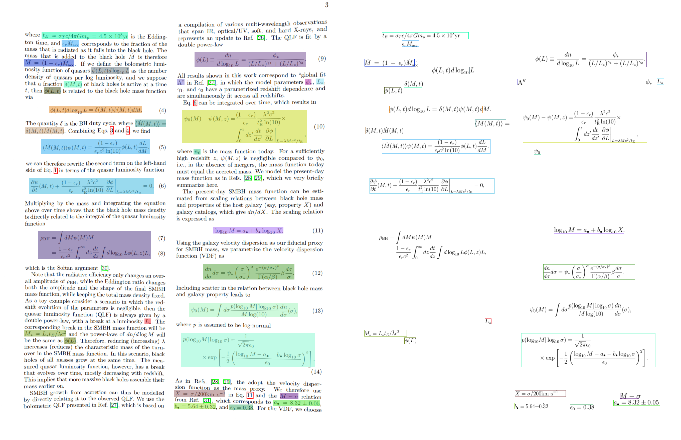
{'res': {'input_path': './general_formula_recognition_001.png', 'page_index': None, 'model_settings': {'use_doc_preprocessor': True, 'use_layout_detection': True}, 'doc_preprocessor_res': {'input_path': None, 'page_index': None, 'model_settings': {'use_doc_orientation_classify': True, 'use_doc_unwarping': True}, 'angle': 0}, 'layout_det_res': {'input_path': None, 'page_index': None, 'boxes': [{'cls_id': 2, 'label': 'text', 'score': 0.9855189323425293, 'coordinate': [90.56131, 1086.7773, 658.8992, 1553.2681]}, {'cls_id': 2, 'label': 'text', 'score': 0.9814704060554504, 'coordinate': [93.04651, 127.988556, 664.8587, 396.60892]}, {'cls_id': 2, 'label': 'text', 'score': 0.9767388105392456, 'coordinate': [698.4391, 591.0454, 1293.3676, 748.28345]}, {'cls_id': 2, 'label': 'text', 'score': 0.9712911248207092, 'coordinate': [701.4946, 286.61566, 1299.0099, 391.87457]}, {'cls_id': 2, 'label': 'text', 'score': 0.9709068536758423, 'coordinate': [697.0126, 751.93604, 1290.2236, 883.64453]}, {'cls_id': 2, 'label': 'text', 'score': 0.9689271450042725, 'coordinate': [704.01196, 79.645935, 1304.7493, 187.96674]}, {'cls_id': 2, 'label': 'text', 'score': 0.9683637619018555, 'coordinate': [93.063385, 799.3567, 660.6935, 902.0344]}, {'cls_id': 7, 'label': 'formula', 'score': 0.9660536646842957, 'coordinate': [728.5045, 440.9215, 1224.0634, 570.8518]}, {'cls_id': 7, 'label': 'formula', 'score': 0.9616329669952393, 'coordinate': [722.9789, 1333.5085, 1257.1136, 1468.0432]}, {'cls_id': 7, 'label': 'formula', 'score': 0.9610316753387451, 'coordinate': [756.4525, 1211.323, 1188.0428, 1268.2336]}, {'cls_id': 7, 'label': 'formula', 'score': 0.960993230342865, 'coordinate': [777.51355, 207.87927, 1222.8966, 267.33014]}, {'cls_id': 2, 'label': 'text', 'score': 0.9594196677207947, 'coordinate': [697.5154, 957.6764, 1288.6238, 1033.5211]}, {'cls_id': 2, 'label': 'text', 'score': 0.9593432545661926, 'coordinate': [691.333, 1511.8015, 1282.0968, 1642.5906]}, {'cls_id': 7, 'label': 'formula', 'score': 0.9589930176734924, 'coordinate': [153.89856, 924.2046, 601.0946, 1036.9038]}, {'cls_id': 2, 'label': 'text', 'score': 0.9582098722457886, 'coordinate': [87.02347, 1557.2971, 655.9584, 1632.6912]}, {'cls_id': 7, 'label': 'formula', 'score': 0.9579620957374573, 'coordinate': [810.86975, 1057.0771, 1175.101, 1117.6631]}, {'cls_id': 7, 'label': 'formula', 'score': 0.9557801485061646, 'coordinate': [165.26271, 557.8495, 598.1803, 614.35]}, {'cls_id': 7, 'label': 'formula', 'score': 0.953873872756958, 'coordinate': [116.48187, 713.88416, 614.2181, 774.02576]}, {'cls_id': 2, 'label': 'text', 'score': 0.9521227478981018, 'coordinate': [96.6882, 478.32745, 662.573, 536.5877]}, {'cls_id': 2, 'label': 'text', 'score': 0.944242000579834, 'coordinate': [96.12866, 639.1591, 661.7959, 692.4849]}, {'cls_id': 2, 'label': 'text', 'score': 0.9403323531150818, 'coordinate': [695.9436, 1138.6748, 1286.7242, 1188.0049]}, {'cls_id': 7, 'label': 'formula', 'score': 0.9249663949012756, 'coordinate': [852.90137, 908.64386, 1131.1882, 933.81793]}, {'cls_id': 7, 'label': 'formula', 'score': 0.9249223470687866, 'coordinate': [195.28397, 424.81024, 567.697, 451.1291]}, {'cls_id': 17, 'label': 'formula_number', 'score': 0.9173304438591003, 'coordinate': [1246.2393, 1079.0535, 1286.3281, 1104.3323]}, {'cls_id': 17, 'label': 'formula_number', 'score': 0.9169507026672363, 'coordinate': [1246.9003, 908.6482, 1288.2013, 934.61426]}, {'cls_id': 17, 'label': 'formula_number', 'score': 0.915979266166687, 'coordinate': [1247.0374, 1229.1572, 1287.094, 1254.9805]}, {'cls_id': 17, 'label': 'formula_number', 'score': 0.9085646867752075, 'coordinate': [1252.864, 492.1079, 1294.6238, 518.47095]}, {'cls_id': 17, 'label': 'formula_number', 'score': 0.9017605781555176, 'coordinate': [1242.1719, 1473.6951, 1283.02, 1498.6316]}, {'cls_id': 17, 'label': 'formula_number', 'score': 0.8999755382537842, 'coordinate': [1269.8164, 220.34933, 1299.8589, 247.01102]}, {'cls_id': 7, 'label': 'formula', 'score': 0.8965252041816711, 'coordinate': [96.00711, 235.49493, 295.43823, 265.60016]}, {'cls_id': 2, 'label': 'text', 'score': 0.8954343199729919, 'coordinate': [696.85693, 1286.2236, 1083.3921, 1310.8643]}, {'cls_id': 7, 'label': 'formula', 'score': 0.8952110409736633, 'coordinate': [166.60979, 129.20242, 511.65692, 156.29672]}, {'cls_id': 2, 'label': 'text', 'score': 0.893648624420166, 'coordinate': [725.64575, 396.18964, 1263.0391, 422.76813]}, {'cls_id': 17, 'label': 'formula_number', 'score': 0.8922948837280273, 'coordinate': [634.14124, 427.77087, 661.1686, 454.10022]}, {'cls_id': 2, 'label': 'text', 'score': 0.8892256617546082, 'coordinate': [94.483246, 1058.7595, 441.92313, 1082.4875]}, {'cls_id': 17, 'label': 'formula_number', 'score': 0.8878197073936462, 'coordinate': [630.4175, 939.3015, 657.7135, 965.36426]}, {'cls_id': 17, 'label': 'formula_number', 'score': 0.8831961154937744, 'coordinate': [630.5835, 1000.95715, 657.4309, 1026.2128]}, {'cls_id': 17, 'label': 'formula_number', 'score': 0.8767948150634766, 'coordinate': [634.1024, 575.3833, 660.59094, 601.1677]}, {'cls_id': 7, 'label': 'formula', 'score': 0.873543918132782, 'coordinate': [95.29655, 1320.3627, 264.93008, 1345.8473]}, {'cls_id': 17, 'label': 'formula_number', 'score': 0.8702306151390076, 'coordinate': [633.82825, 730.31525, 659.83215, 755.5485]}, {'cls_id': 7, 'label': 'formula', 'score': 0.8387619853019714, 'coordinate': [365.19897, 268.29675, 515.7938, 296.07013]}, {'cls_id': 7, 'label': 'formula', 'score': 0.8314349055290222, 'coordinate': [1090.509, 1599.1382, 1276.6736, 1622.156]}, {'cls_id': 7, 'label': 'formula', 'score': 0.817135751247406, 'coordinate': [246.175, 161.22958, 314.3764, 186.40591]}, {'cls_id': 3, 'label': 'number', 'score': 0.8042846322059631, 'coordinate': [1297.4036, 7.1497707, 1310.5969, 27.737753]}, {'cls_id': 7, 'label': 'formula', 'score': 0.7970448136329651, 'coordinate': [538.45593, 478.09354, 661.8812, 508.50778]}, {'cls_id': 7, 'label': 'formula', 'score': 0.7644855976104736, 'coordinate': [916.51746, 1618.5188, 1009.62537, 1640.8206]}, {'cls_id': 7, 'label': 'formula', 'score': 0.7423419952392578, 'coordinate': [694.8439, 1612.2507, 861.05334, 1635.9768]}, {'cls_id': 7, 'label': 'formula', 'score': 0.7072376608848572, 'coordinate': [99.72007, 508.21167, 254.91953, 535.74744]}, {'cls_id': 7, 'label': 'formula', 'score': 0.6976271867752075, 'coordinate': [696.8011, 1561.4375, 899.79584, 1586.7349]}, {'cls_id': 7, 'label': 'formula', 'score': 0.6707713007926941, 'coordinate': [1117.0862, 1571.9763, 1191.502, 1594.742]}, {'cls_id': 7, 'label': 'formula', 'score': 0.6338322162628174, 'coordinate': [577.33484, 1274.4131, 602.5636, 1296.7021]}, {'cls_id': 7, 'label': 'formula', 'score': 0.6199935674667358, 'coordinate': [175.28284, 349.82376, 241.24683, 376.6708]}, {'cls_id': 7, 'label': 'formula', 'score': 0.612853467464447, 'coordinate': [773.06287, 595.202, 800.43884, 617.3812]}, {'cls_id': 7, 'label': 'formula', 'score': 0.6107096672058105, 'coordinate': [706.6776, 316.87082, 736.69714, 339.9352]}, {'cls_id': 7, 'label': 'formula', 'score': 0.5520269870758057, 'coordinate': [1263.9711, 314.65167, 1292.7728, 337.3896]}, {'cls_id': 7, 'label': 'formula', 'score': 0.5346108675003052, 'coordinate': [1219.2955, 316.599, 1243.9181, 339.71802]}, {'cls_id': 7, 'label': 'formula', 'score': 0.5195119380950928, 'coordinate': [254.65729, 323.6553, 326.57758, 349.53494]}, {'cls_id': 7, 'label': 'formula', 'score': 0.501812219619751, 'coordinate': [255.8518, 1350.6472, 301.74304, 1375.5286]}]}, 'formula_res_list': [{'rec_formula': '\\begin{aligned}{\\psi_{0}(M)-\\psi_{}(M,z)=}&{{}\\frac{(1-\\epsilon_{r})}{\\epsilon_{r}}\\frac{\\lambda^{2}c^{2}}{t_{\\operatorname{E}}^{2}\\operatorname{l n}(10)}\\times}\\\\ {}&{{}\\int_{0}^{z}d z^{\\prime}\\frac{d t}{d z^{\\prime}}\\left.\\frac{\\partial\\phi}{\\partial L}\\right|_{L=\\lambda M c^{2}/t_{\\operatorname{E}}},}\\\\ \\end{aligned}', 'formula_region_id': 1, 'dt_polys': ([728.5045, 440.9215, 1224.0634, 570.8518],)}, {'rec_formula': '\\begin{aligned}{p(\\operatorname{l o g}_{10}}&{{}M|\\operatorname{l o g}_{10}\\sigma)=\\frac{1}{\\sqrt{2\\pi}\\epsilon_{0}}}\\\\ {}&{{}\\times\\operatorname{e x p}\\left[-\\frac{1}{2}\\left(\\frac{\\operatorname{l o g}_{10}M-a_{\\bullet}-b_{\\bullet}\\operatorname{l o g}_{10}\\sigma}{\\epsilon_{0}}\\right)^{2}\\right].}\\\\ \\end{aligned}', 'formula_region_id': 2, 'dt_polys': ([722.9789, 1333.5085, 1257.1136, 1468.0432],)}, {'rec_formula': '\\psi_{0}(M)=\\int d\\sigma\\frac{p(\\operatorname{l o g}_{10}M|\\operatorname{l o g}_{10}\\sigma)}{M\\operatorname{l o g}(10)}\\frac{d n}{d\\sigma}(\\sigma),', 'formula_region_id': 3, 'dt_polys': ([756.4525, 1211.323, 1188.0428, 1268.2336],)}, {'rec_formula': '\\phi(L)\\equiv\\frac{d n}{d\\operatorname{l o g}_{10}L}=\\frac{\\phi_{*}}{(L/L_{*})^{\\gamma_{1}}+(L/L_{*})^{\\gamma_{2}}}.', 'formula_region_id': 4, 'dt_polys': ([777.51355, 207.87927, 1222.8966, 267.33014],)}, {'rec_formula': '\\begin{aligned}{\\rho_{\\operatorname{B H}}}&{{}=\\int d M\\psi(M)M}\\\\ {}&{{}=\\frac{1-\\epsilon_{r}}{\\epsilon_{r}c^{2}}\\int_{0}^{\\infty}d z\\frac{d t}{d z}\\int d\\operatorname{l o g}_{10}L\\phi(L,z)L,}\\\\ \\end{aligned}', 'formula_region_id': 5, 'dt_polys': ([153.89856, 924.2046, 601.0946, 1036.9038],)}, {'rec_formula': '\\frac{d n}{d\\sigma}d\\sigma=\\psi_{*}\\left(\\frac{\\sigma}{\\sigma_{*}}\\right)^{\\alpha}\\frac{e^{-(\\sigma/\\sigma_{*})^{\\beta}}}{\\Gamma(\\alpha/\\beta)}\\beta\\frac{d\\sigma}{\\sigma}.', 'formula_region_id': 6, 'dt_polys': ([810.86975, 1057.0771, 1175.101, 1117.6631],)}, {'rec_formula': '\\langle\\dot{M}(M,t)\\rangle\\psi(M,t)=\\frac{(1-\\epsilon_{r})}{\\epsilon_{r}c^{2}\\operatorname{l n}(10)}\\phi(L,t)\\frac{d L}{d M}.', 'formula_region_id': 7, 'dt_polys': ([165.26271, 557.8495, 598.1803, 614.35],)}, {'rec_formula': '\\frac{\\partial\\psi}{\\partial t}(M,t)+\\frac{(1-\\epsilon_{r})}{\\epsilon_{r}}\\frac{\\lambda^{2}c^{2}}{t_{\\operatorname{E}}^{2}\\operatorname{l n}(10)}\\left.\\frac{\\partial\\phi}{\\partial L}\\right|_{L=\\lambda M c^{2}/t_{\\operatorname{E}}}=0,', 'formula_region_id': 8, 'dt_polys': ([116.48187, 713.88416, 614.2181, 774.02576],)}, {'rec_formula': '\\operatorname{l o g}_{10}M=a_{\\bullet}+b_{\\bullet}\\operatorname{l o g}_{10}X.', 'formula_region_id': 9, 'dt_polys': ([852.90137, 908.64386, 1131.1882, 933.81793],)}, {'rec_formula': '\\phi(L,t)d\\operatorname{l o g}_{10}L=\\delta(M,t)\\psi(M,t)d M.', 'formula_region_id': 10, 'dt_polys': ([195.28397, 424.81024, 567.697, 451.1291],)}, {'rec_formula': '\\dot{M}\\:=\\:(1\\:-\\:\\epsilon_{r})\\dot{M}_{\\mathrm{a c c}}^{\\mathrm{~\\tiny~\\cdot~}}', 'formula_region_id': 11, 'dt_polys': ([96.00711, 235.49493, 295.43823, 265.60016],)}, {'rec_formula': 't_{E}=\\sigma_{T}c/4\\pi G m_{p}=4.5\\times10^{8}\\mathrm{y r}', 'formula_region_id': 12, 'dt_polys': ([166.60979, 129.20242, 511.65692, 156.29672],)}, {'rec_formula': 'M_{*}=L_{*}t_{E}/\\tilde{\\lambda}c^{2}', 'formula_region_id': 13, 'dt_polys': ([95.29655, 1320.3627, 264.93008, 1345.8473],)}, {'rec_formula': '\\phi(L,t)d\\operatorname{l o g}_{10}L', 'formula_region_id': 14, 'dt_polys': ([365.19897, 268.29675, 515.7938, 296.07013],)}, {'rec_formula': 'a_{\\bullet}=8.32\\pm0.05', 'formula_region_id': 15, 'dt_polys': ([1090.509, 1599.1382, 1276.6736, 1622.156],)}, {'rec_formula': '\\epsilon_{r}\\dot{M}_{\\mathrm{a c c}}', 'formula_region_id': 16, 'dt_polys': ([246.175, 161.22958, 314.3764, 186.40591],)}, {'rec_formula': '\\langle\\dot{M}(M,t)\\rangle=', 'formula_region_id': 17, 'dt_polys': ([538.45593, 478.09354, 661.8812, 508.50778],)}, {'rec_formula': '\\epsilon_{0}=0.38', 'formula_region_id': 18, 'dt_polys': ([916.51746, 1618.5188, 1009.62537, 1640.8206],)}, {'rec_formula': 'b_{\\bullet}=5.64\\dot{\\pm}\\dot{0.32}', 'formula_region_id': 19, 'dt_polys': ([694.8439, 1612.2507, 861.05334, 1635.9768],)}, {'rec_formula': '\\delta(M,t)\\dot{M}(M,t)', 'formula_region_id': 20, 'dt_polys': ([99.72007, 508.21167, 254.91953, 535.74744],)}, {'rec_formula': 'X=\\sigma/200\\mathrm{k m}\\mathrm{~s^{-1}~}', 'formula_region_id': 21, 'dt_polys': ([696.8011, 1561.4375, 899.79584, 1586.7349],)}, {'rec_formula': 'M-\\sigma', 'formula_region_id': 22, 'dt_polys': ([1117.0862, 1571.9763, 1191.502, 1594.742],)}, {'rec_formula': 'L_{*}', 'formula_region_id': 23, 'dt_polys': ([577.33484, 1274.4131, 602.5636, 1296.7021],)}, {'rec_formula': '\\phi(L,t)', 'formula_region_id': 24, 'dt_polys': ([175.28284, 349.82376, 241.24683, 376.6708],)}, {'rec_formula': '\\psi_{0}', 'formula_region_id': 25, 'dt_polys': ([773.06287, 595.202, 800.43884, 617.3812],)}, {'rec_formula': '\\mathrm{A^{\\prime\\prime}}', 'formula_region_id': 26, 'dt_polys': ([706.6776, 316.87082, 736.69714, 339.9352],)}, {'rec_formula': 'L_{*}', 'formula_region_id': 27, 'dt_polys': ([1263.9711, 314.65167, 1292.7728, 337.3896],)}, {'rec_formula': '\\phi_{*}', 'formula_region_id': 28, 'dt_polys': ([1219.2955, 316.599, 1243.9181, 339.71802],)}, {'rec_formula': '\\delta(M,t)', 'formula_region_id': 29, 'dt_polys': ([254.65729, 323.6553, 326.57758, 349.53494],)}, {'rec_formula': '\\phi(L)', 'formula_region_id': 30, 'dt_polys': ([255.8518, 1350.6472, 301.74304, 1375.5286],)}]}}
运行结果参数说明可以参考2.2 Python脚本方式集成中的结果解释。
可视化结果保存在save_path下,其中公式识别的可视化结果如下:
如果您需要对公式识别产线进行可视化,需要运行如下命令来对LaTeX渲染环境进行安装。目前公式识别产线可视化只支持Ubuntu环境,其他环境暂不支持。对于复杂公式,LaTeX 结果可能包含部分高级的表示,Markdown等环境中未必可以成功显示:
sudo apt-get update
sudo apt-get install texlive texlive-latex-base texlive-xetex latex-cjk-all texlive-latex-extra -y
备注: 由于公式识别可视化过程中需要对每张公式图片进行渲染,因此耗时较长,请您耐心等待。
2.2 Python脚本方式集成
命令行方式是为了快速体验查看效果,一般来说,在项目中,往往需要通过代码集成,您可以通过几行代码即可完成产线的快速推理,推理代码如下:
from paddleocr import FormulaRecognitionPipeline

pipeline = FormulaRecognitionPipeline()
# ocr = FormulaRecognitionPipeline(use_doc_orientation_classify=True) # 通过 use_doc_orientation_classify 指定是否使用文档方向分类模型
# ocr = FormulaRecognitionPipeline(use_doc_unwarping=True) # 通过 use_doc_unwarping 指定是否使用文本图像矫正模块
# ocr = FormulaRecognitionPipeline(device="gpu") # 通过 device 指定模型推理时使用 GPU
output = pipeline.predict("./general_formula_recognition_001.png")
for res in output:
    res.print() ## 打印预测的结构化输出
    res.save_to_img(save_path="output") ## 保存当前图像的公式可视化结果
    res.save_to_json(save_path="output") ## 保存当前图像的结构化json结果
在上述 Python 脚本中,执行了如下几个步骤:
(1)通过 FormulaRecognitionPipeline() 实例化公式识别产线对象,具体参数说明如下:
| 参数 | 参数说明 | 参数类型 | 默认值 |
|---|---|---|---|
doc_orientation_classify_model_name |
文档方向分类模型的名称。如果设置为None,将会使用产线默认模型。 |
str|None |
None |
doc_orientation_classify_model_dir |
文档方向分类模型的目录路径。如果设置为None,将会下载官方模型。 |
str|None |
None |
doc_orientation_classify_batch_size |
文档方向分类模型的batch size。如果设置为None,将默认设置batch size为1。 |
int|None |
None |
doc_unwarping_model_name |
文本图像矫正模型的名称。如果设置为None,将会使用产线默认模型。 |
str|None |
None |
doc_unwarping_model_dir |
文本图像矫正模型的目录路径。如果设置为None,将会下载官方模型。 |
str|None |
None |
doc_unwarping_batch_size |
文本图像矫正模型的batch size。如果设置为None,将默认设置batch size为1。 |
int|None |
None |
use_doc_orientation_classify |
是否加载并使用文档方向分类模块。如果设置为None,将使用产线初始化的该参数值,默认初始化为True。 |
bool|None |
None |
use_doc_unwarping |
是否加载并使用文本图像矫正模块。如果设置为None,将使用产线初始化的该参数值,默认初始化为True。 |
bool|None |
None |
layout_detection_model_name |
版面区域检测模型的名称。如果设置为None,将会使用产线默认模型。 |
str|None |
None |
layout_detection_model_dir |
版面区域检测模型的目录路径。如果设置为None,将会下载官方模型。 |
str|None |
None |
layout_threshold |
版面区域检测的阈值,用于过滤掉低置信度预测结果的阈值。
|
float|dict|None |
None |
layout_nms |
版面检测是否使用后处理NMS。如果不设置,将使用产线初始化的该参数值,默认初始化为True。 |
bool|None |
None |
layout_unclip_ratio |
版面区域检测模型检测框的扩张系数。
|
float|Tuple[float,float]|dict|None |
None |
layout_merge_bboxes_mode |
版面区域检测的重叠框过滤方式。
|
str|dict|None |
None |
layout_detection_batch_size |
版面区域检测模型的batch size。如果设置为None,将默认设置batch size为1。 |
int|None |
None |
use_layout_detection |
是否加载并使用版面区域检测模块。如果设置为None,将使用产线初始化的该参数值,默认初始化为True。 |
bool|None |
None |
formula_recognition_model_name |
公式识别模型的名称。如果设置为None,将会使用产线默认模型。 |
str|None |
None |
formula_recognition_model_dir |
公式识别模型的目录路径。如果设置为None,将会下载官方模型。 |
str|None |
None |
formula_recognition_batch_size |
公式识别模型的batch size。如果设置为None,将默认设置batch size为1。 |
int|None |
None |
device |
用于推理的设备。支持指定具体卡号:
|
str|None |
None |
enable_hpi |
是否启用高性能推理。 | bool |
False |
use_tensorrt |
是否启用 Paddle Inference 的 TensorRT 子图引擎。如果模型不支持通过 TensorRT 加速,即使设置了此标志,也不会使用加速。 对于 CUDA 11.8 版本的飞桨,兼容的 TensorRT 版本为 8.x(x>=6),建议安装 TensorRT 8.6.1.6。 |
bool |
False |
precision |
计算精度,如 fp32、fp16。 | str |
"fp32" |
enable_mkldnn |
是否启用 MKL-DNN 加速推理。如果 MKL-DNN 不可用或模型不支持通过 MKL-DNN 加速,即使设置了此标志,也不会使用加速。 | bool |
True |
mkldnn_cache_capacity |
MKL-DNN 缓存容量。 | int |
10 |
cpu_threads |
在 CPU 上进行推理时使用的线程数。 | int |
8 |
paddlex_config |
PaddleX产线配置文件路径。 | str|None |
None |
(2)调用 公式识别产线对象的 predict() 方法进行推理预测,该方法会返回一个结果列表。
另外,产线还提供了 predict_iter() 方法。两者在参数接受和结果返回方面是完全一致的,区别在于 predict_iter() 返回的是一个 generator,能够逐步处理和获取预测结果,适合处理大型数据集或希望节省内存的场景。可以根据实际需求选择使用这两种方法中的任意一种。
以下是 predict() 方法的参数及其说明:
| 参数 | 参数说明 | 参数类型 | 默认值 |
|---|---|---|---|
input |
待预测数据,支持多种输入类型,必填
|
Python Var|str|list |
|
use_layout_detection |
是否在推理时使用文档区域检测模块。 | bool|None |
None |
use_doc_orientation_classify |
是否在推理时使用文档方向分类模块。 | bool|None |
None |
use_doc_unwarping |
是否在推理时使用文本图像矫正模块。 | bool|None |
None |
layout_threshold |
参数含义与实例化参数基本相同。设置为None表示使用实例化参数,否则该参数优先级更高。 |
float|dict|None |
None |
layout_nms |
参数含义与实例化参数基本相同。设置为None表示使用实例化参数,否则该参数优先级更高。 |
bool|None |
None |
layout_unclip_ratio |
参数含义与实例化参数基本相同。设置为None表示使用实例化参数,否则该参数优先级更高。 |
float|Tuple[float,float]|dict|None |
None |
layout_merge_bboxes_mode |
参数含义与实例化参数基本相同。设置为None表示使用实例化参数,否则该参数优先级更高。 |
str|dict|None |
None |
(3)对预测结果进行处理,每个样本的预测结果均为对应的Result对象,且支持打印、保存为图片、保存为json文件的操作:
| 方法 | 方法说明 | 参数 | 参数类型 | 参数说明 | 默认值 |
|---|---|---|---|---|---|
print() |
打印结果到终端 | format_json |
bool |
是否对输出内容进行使用 JSON 缩进格式化。 |
True |
indent |
int |
指定缩进级别,以美化输出的 JSON 数据,使其更具可读性,仅当 format_json 为 True 时有效。 |
4 | ||
ensure_ascii |
bool |
控制是否将非 ASCII 字符转义为 Unicode。设置为 True 时,所有非 ASCII 字符将被转义;False 则保留原始字符,仅当format_json为True时有效。 |
False |
||
save_to_json() |
将结果保存为json格式的文件 | save_path |
str |
保存的文件路径,当为目录时,保存文件命名与输入文件类型命名一致。 | 无 |
indent |
int |
指定缩进级别,以美化输出的 JSON 数据,使其更具可读性,仅当 format_json 为 True 时有效。 |
4 | ||
ensure_ascii |
bool |
控制是否将非 ASCII 字符转义为 Unicode。设置为 True 时,所有非 ASCII 字符将被转义;False 则保留原始字符,仅当format_json为True时有效。 |
False |
||
save_to_img() |
将结果保存为图像格式的文件 | save_path |
str |
保存的文件路径,支持目录或文件路径。 | 无 |
-
调用
print()方法会将结果打印到终端,打印到终端的内容解释如下:-
input_path:(str)待预测图像的输入路径 -
page_index:(Union[int, None])如果输入是PDF文件,则表示当前是PDF的第几页,否则为None -
model_settings:(Dict[str, bool])配置产线所需的模型参数use_doc_preprocessor:(bool)控制是否启用文档预处理子产线use_layout_detection:(bool)控制是否启用版面区域检测模块
-
doc_preprocessor_res:(Dict[str, Union[str, Dict[str, bool], int]])文档预处理子产线的输出结果。仅当use_doc_preprocessor=True时存在input_path:(Union[str, None])图像预处理子产线接受的图像路径,当输入为numpy.ndarray时,保存为Nonemodel_settings:(Dict)预处理子产线的模型配置参数use_doc_orientation_classify:(bool)控制是否启用文档方向分类use_doc_unwarping:(bool)控制是否启用文本图像矫正
angle:(int)文档方向分类的预测结果。启用时取值为[0,1,2,3],分别对应[0°,90°,180°,270°];未启用时为-1
layout_det_res:(Dict[str, List[Dict]])版面区域检测模块的输出结果。仅当use_layout_detection=True时存在input_path:(Union[str, None])版面区域检测模块接收的图像路径,当输入为numpy.ndarray时,保存为Noneboxes:(List[Dict[int, str, float, List[float]]])版面区域检测预测结果列表cls_id:(int)版面区域检测预测的类别idlabel:(str)版面区域检测预测的类别score:(float)版面区域检测预测的类别置信度分数coordinate:(List[float])版面区域检测预测的边界框坐标,格式为[x_min, y_min, x_max, y_max],其中(x_min, y_min)为左上角坐标,(x_max, y_max) 为右上角坐标
formula_res_list:(List[Dict[str, int, List[float]]])公式识别的预测结果列表rec_formula:(str)公式识别预测的LaTeX源码formula_region_id:(int)公式识别预测的id编号dt_polys:(List[float])公式识别预测的边界框坐标,格式为[x_min, y_min, x_max, y_max],其中(x_min, y_min)为左上角坐标,(x_max, y_max) 为右上角坐标
-
-
调用
save_to_json()方法会将上述内容保存到指定的save_path中,如果指定为目录,则保存的路径为save_path/{your_img_basename}_res.json,如果指定为文件,则直接保存到该文件中。由于json文件不支持保存numpy数组,因此会将其中的numpy.array类型转换为列表形式。 -
调用
save_to_img()方法会将可视化结果保存到指定的save_path中,如果指定为目录,则保存的路径为save_path/{your_img_basename}_formula_res_img.{your_img_extension},如果指定为文件,则直接保存到该文件中。(产线通常包含较多结果图片,不建议直接指定为具体的文件路径,否则多张图会被覆盖,仅保留最后一张图) -
此外,也支持通过属性获取带结果的可视化图像和预测结果,具体如下:
| 属性 | 属性说明 |
|---|---|
json |
获取预测的 json 格式的结果 |
img |
获取格式为 dict 的可视化图像 |
json属性获取的预测结果为dict类型的数据,相关内容与调用save_to_json()方法保存的内容一致。img属性返回的预测结果是一个dict类型的数据。其中,键分别为preprocessed_img、layout_det_res和formula_res_img,对应的值是三个Image.Image对象:第一个用于展示图像预处理的可视化图像,第二个用于展示版面区域检测的可视化图像,第三个用于展示公式识别的可视化图像。如果没有使用图像预处理子模块,则dict中不包含preprocessed_img;如果没有使用版面区域检测子模块,则dict中不包含layout_det_res。
3. 开发集成/部署
如果产线可以达到您对产线推理速度和精度的要求,您可以直接进行开发集成/部署。
若您需要将产线直接应用在您的Python项目中,可以参考 2.2 Python脚本方式中的示例代码。
此外,PaddleOCR 也提供了其他两种部署方式,详细说明如下:
🚀 高性能推理:在实际生产环境中,许多应用对部署策略的性能指标(尤其是响应速度)有着较严苛的标准,以确保系统的高效运行与用户体验的流畅性。为此,PaddleOCR 提供高性能推理功能,旨在对模型推理及前后处理进行深度性能优化,实现端到端流程的显著提速,详细的高性能推理流程请参考高性能推理。
☁️ 服务化部署:服务化部署是实际生产环境中常见的一种部署形式。通过将推理功能封装为服务,客户端可以通过网络请求来访问这些服务,以获取推理结果。详细的产线服务化部署流程请参考服务化部署。
以下是基础服务化部署的API参考与多语言服务调用示例:
API参考
对于服务提供的主要操作:
- HTTP请求方法为POST。
- 请求体和响应体均为JSON数据(JSON对象)。
- 当请求处理成功时,响应状态码为
200,响应体的属性如下:
| 名称 | 类型 | 含义 |
|---|---|---|
logId |
string |
请求的UUID。 |
errorCode |
integer |
错误码。固定为0。 |
errorMsg |
string |
错误说明。固定为"Success"。 |
result |
object |
操作结果。 |
- 当请求处理未成功时,响应体的属性如下:
| 名称 | 类型 | 含义 |
|---|---|---|
logId |
string |
请求的UUID。 |
errorCode |
integer |
错误码。与响应状态码相同。 |
errorMsg |
string |
错误说明。 |
服务提供的主要操作如下:
infer
获取图像公式识别结果。
POST /formula-recognition
- 请求体的属性如下:
| 名称 | 类型 | 含义 | 是否必填 |
|---|---|---|---|
file |
string |
服务器可访问的图像文件或PDF文件的URL,或上述类型文件内容的Base64编码结果。默认对于超过10页的PDF文件,只有前10页的内容会被处理。 要解除页数限制,请在产线配置文件中添加以下配置: |
是 |
fileType |
integer | null |
文件类型。0表示PDF文件,1表示图像文件。若请求体无此属性,则将根据URL推断文件类型。 |
否 |
useDocOrientationClassify |
boolean | null |
请参阅产线对象中 predict 方法的 use_doc_orientation_classify 参数相关说明。 |
否 |
useDocUnwarping |
boolean | null |
请参阅产线对象中 predict 方法的 use_doc_unwarping 参数相关说明。 |
否 |
useLayoutDetection |
boolean | null |
请参阅产线对象中 predict方法的 use_layout_detection 参数相关说明。 |
否 |
layoutThreshold |
number | null |
请参阅产线对象中predict 法的layout_threshold 参数相关说明。 |
否 |
layoutNms |
boolean | null |
请参阅产线对象中predict 法的layout_nms 参数相关说明。 |
否 |
layoutUnclipRatio |
number | array | null |
请参阅产线对象中 predict方法的 layout_unclip_ratio 参数相关说明。 |
否 |
layoutMergeBboxesMode |
string | null |
请参阅产线对象中predict方法的 layout_merge_bboxes_mode 参数相关说明。 |
否 |
visualize |
boolean | null |
是否返回可视化结果图以及处理过程中的中间图像等。
例如,在产线配置文件中添加如下字段: visualize参数可以覆盖默认行为。如果请求体和配置文件中均未设置(或请求体传入null、配置文件中未设置),则默认返回图像。
|
否 |
- 请求处理成功时,响应体的
result具有如下属性:
| 名称 | 类型 | 含义 |
|---|---|---|
formulaRecResults |
object |
公式识别结果。数组长度为1(对于图像输入)或实际处理的文档页数(对于PDF输入)。对于PDF输入,数组中的每个元素依次表示PDF文件中实际处理的每一页的结果。 |
dataInfo |
object |
输入数据信息。 |
formulaRecResults中的每个元素为一个object,具有如下属性:
| 名称 | 类型 | 含义 |
|---|---|---|
prunedResult |
object |
产线对象的 predict 方法生成结果的JSON表示中res字段的简化版本,其中去除了input_path和 page_index字段。 |
outputImages |
object | null |
参见产线预测结果的img属性说明。图像为JPEG格式,使用Base64编码。 |
inputImage | null |
string |
输入图像。图像为JPEG格式,使用Base64编码。 |
多语言调用服务示例
Python
import base64
import requests

API_URL = "http://localhost:8080/formula-recognition"
file_path = "./demo.jpg"

with open(file_path, "rb") as file:
    file_bytes = file.read()
    file_data = base64.b64encode(file_bytes).decode("ascii")

payload = {"file": file_data, "fileType": 1}

response = requests.post(API_URL, json=payload)

assert response.status_code == 200
result = response.json()["result"]
for i, res in enumerate(result["formulaRecResults"]):
    print(res["prunedResult"])
    for img_name, img in res["outputImages"].items():
        img_path = f"{img_name}_{i}.jpg"
        with open(img_path, "wb") as f:
            f.write(base64.b64decode(img))
        print(f"Output image saved at {img_path}")
C++
#include <iostream>
#include <fstream>
#include <vector>
#include <string>
#include "cpp-httplib/httplib.h" // https://github.com/Huiyicc/cpp-httplib
#include "nlohmann/json.hpp" // https://github.com/nlohmann/json
#include "base64.hpp" // https://github.com/tobiaslocker/base64

int main() {
    httplib::Client client("localhost", 8080);

    const std::string filePath = "./demo.jpg";

    std::ifstream file(filePath, std::ios::binary | std::ios::ate);
    if (!file) {
        std::cerr << "Error opening file: " << filePath << std::endl;
        return 1;
    }

    std::streamsize size = file.tellg();
    file.seekg(0, std::ios::beg);
    std::vector buffer(size);
    if (!file.read(buffer.data(), size)) {
        std::cerr << "Error reading file." << std::endl;
        return 1;
    }

    std::string bufferStr(buffer.data(), static_cast(size));
    std::string encodedFile = base64::to_base64(bufferStr);

    nlohmann::json jsonObj;
    jsonObj["file"] = encodedFile;
    jsonObj["fileType"] = 1;

    auto response = client.Post("/formula-recognition", jsonObj.dump(), "application/json");

    if (response && response->status == 200) {
        nlohmann::json jsonResponse = nlohmann::json::parse(response->body);
        auto result = jsonResponse["result"];

        if (!result.is_object() || !result["formulaRecResults"].is_array()) {
            std::cerr << "Unexpected response format." << std::endl;
            return 1;
        }

        for (size_t i = 0; i < result["formulaRecResults"].size(); ++i) {
            auto res = result["formulaRecResults"][i];

            if (res.contains("prunedResult")) {
                std::cout << "Recognized formula: " << res["prunedResult"].dump() << std::endl;
            }

            if (res.contains("outputImages") && res["outputImages"].is_object()) {
                for (auto& [imgName, imgData] : res["outputImages"].items()) {
                    std::string outputPath = imgName + "_" + std::to_string(i) + ".jpg";
                    std::string decodedImage = base64::from_base64(imgData.get());

                    std::ofstream outFile(outputPath, std::ios::binary);
                    if (outFile.is_open()) {
                        outFile.write(decodedImage.c_str(), decodedImage.size());
                        outFile.close();
                        std::cout << "Saved image: " << outputPath << std::endl;
                    } else {
                        std::cerr << "Failed to write image: " << outputPath << std::endl;
                    }
                }
            }
        }
    } else {
        std::cerr << "Request failed." << std::endl;
        if (response) {
            std::cerr << "HTTP status: " << response->status << std::endl;
            std::cerr << "Response body: " << response->body << std::endl;
        }
        return 1;
    }

    return 0;
}
Java
import okhttp3.*;
import com.fasterxml.jackson.databind.ObjectMapper;
import com.fasterxml.jackson.databind.JsonNode;
import com.fasterxml.jackson.databind.node.ObjectNode;

import java.io.File;
import java.io.FileOutputStream;
import java.io.IOException;
import java.util.Base64;

public class Main {
    public static void main(String[] args) throws IOException {
        String API_URL = "http://localhost:8080/formula-recognition";
        String imagePath = "./demo.jpg";

        File file = new File(imagePath);
        byte[] fileContent = java.nio.file.Files.readAllBytes(file.toPath());
        String base64Image = Base64.getEncoder().encodeToString(fileContent);

        ObjectMapper objectMapper = new ObjectMapper();
        ObjectNode payload = objectMapper.createObjectNode();
        payload.put("file", base64Image);
        payload.put("fileType", 1);

        OkHttpClient client = new OkHttpClient();
        MediaType JSON = MediaType.get("application/json; charset=utf-8");
        RequestBody body = RequestBody.create(JSON, payload.toString());

        Request request = new Request.Builder()
                .url(API_URL)
                .post(body)
                .build();

        try (Response response = client.newCall(request).execute()) {
            if (response.isSuccessful()) {
                String responseBody = response.body().string();
                JsonNode root = objectMapper.readTree(responseBody);
                JsonNode result = root.get("result");

                JsonNode formulaRecResults = result.get("formulaRecResults");
                for (int i = 0; i < formulaRecResults.size(); i++) {
                    JsonNode item = formulaRecResults.get(i);
                    int finalI = i;

                    JsonNode prunedResult = item.get("prunedResult");
                    System.out.println("Pruned Result [" + i + "]: " + prunedResult.toString());

                    JsonNode outputImages = item.get("outputImages");
                    if (outputImages != null && outputImages.isObject()) {
                        outputImages.fieldNames().forEachRemaining(imgName -> {
                            try {
                                String imgBase64 = outputImages.get(imgName).asText();
                                byte[] imgBytes = Base64.getDecoder().decode(imgBase64);
                                String imgPath = imgName + "_" + finalI + ".jpg";
                                try (FileOutputStream fos = new FileOutputStream(imgPath)) {
                                    fos.write(imgBytes);
                                    System.out.println("Saved image: " + imgPath);
                                }
                            } catch (IOException e) {
                                System.err.println("Failed to save image: " + e.getMessage());
                            }
                        });
                    }
                }
            } else {
                System.err.println("Request failed with HTTP code: " + response.code());
            }
        }
    }
}
Go
package main

import (
    "bytes"
    "encoding/base64"
    "encoding/json"
    "fmt"
    "io/ioutil"
    "net/http"
    "os"
)

func main() {
    API_URL := "http://localhost:8080/formula-recognition"
    filePath := "./demo.jpg"

    fileBytes, err := ioutil.ReadFile(filePath)
    if err != nil {
        fmt.Printf("Error reading file: %v\n", err)
        return
    }
    fileData := base64.StdEncoding.EncodeToString(fileBytes)

    payload := map[string]interface{}{
        "file":     fileData,
        "fileType": 1,
    }
    payloadBytes, err := json.Marshal(payload)
    if err != nil {
        fmt.Printf("Error marshaling payload: %v\n", err)
        return
    }

    client := &http.Client{}
    req, err := http.NewRequest("POST", API_URL, bytes.NewBuffer(payloadBytes))
    if err != nil {
        fmt.Printf("Error creating request: %v\n", err)
        return
    }
    req.Header.Set("Content-Type", "application/json")

    res, err := client.Do(req)
    if err != nil {
        fmt.Printf("Error sending request: %v\n", err)
        return
    }
    defer res.Body.Close()

    if res.StatusCode != http.StatusOK {
        fmt.Printf("Unexpected status code: %d\n", res.StatusCode)
        return
    }

    body, err := ioutil.ReadAll(res.Body)
    if err != nil {
        fmt.Printf("Error reading response body: %v\n", err)
        return
    }

    type FormulaRecResult struct {
        PrunedResult map[string]interface{} `json:"prunedResult"`
        OutputImages map[string]string      `json:"outputImages"`
        InputImage   *string                `json:"inputImage"`
    }

    type Response struct {
        Result struct {
            FormulaRecResults []FormulaRecResult `json:"formulaRecResults"`
            DataInfo          interface{}        `json:"dataInfo"`
        } `json:"result"`
    }

    var respData Response
    if err := json.Unmarshal(body, &respData); err != nil {
        fmt.Printf("Error unmarshaling response: %v\n", err)
        return
    }

    for i, res := range respData.Result.FormulaRecResults {
        fmt.Printf("Result %d - prunedResult: %+v\n", i, res.PrunedResult)

        for imgName, imgData := range res.OutputImages {
            imgBytes, err := base64.StdEncoding.DecodeString(imgData)
            if err != nil {
                fmt.Printf("Error decoding image %s_%d: %v\n", imgName, i, err)
                continue
            }

            filename := fmt.Sprintf("%s_%d.jpg", imgName, i)
            if err := os.WriteFile(filename, imgBytes, 0644); err != nil {
                fmt.Printf("Error saving image %s: %v\n", filename, err)
                continue
            }
            fmt.Printf("Saved image to %s\n", filename)
        }
    }
}
C#
using System;
using System.IO;
using System.Net.Http;
using System.Text;
using System.Threading.Tasks;
using Newtonsoft.Json.Linq;

class Program
{
    static readonly string API_URL = "http://localhost:8080/formula-recognition";
    static readonly string inputFilePath = "./demo.jpg";

    static async Task Main(string[] args)
    {
        var httpClient = new HttpClient();

        byte[] fileBytes = File.ReadAllBytes(inputFilePath);
        string fileData = Convert.ToBase64String(fileBytes);

        var payload = new JObject
        {
            { "file", fileData },
            { "fileType", 1 }
        };
        var content = new StringContent(payload.ToString(), Encoding.UTF8, "application/json");

        HttpResponseMessage response = await httpClient.PostAsync(API_URL, content);
        response.EnsureSuccessStatusCode();

        string responseBody = await response.Content.ReadAsStringAsync();
        JObject jsonResponse = JObject.Parse(responseBody);

        JArray formulaRecResults = (JArray)jsonResponse["result"]["formulaRecResults"];
        for (int i = 0; i < formulaRecResults.Count; i++)
        {
            var res = formulaRecResults[i];
            Console.WriteLine($"[{i}] prunedResult:\n{res["prunedResult"]}");

            JObject outputImages = res["outputImages"] as JObject;
            if (outputImages != null)
            {
                foreach (var img in outputImages)
                {
                    string imgName = img.Key;
                    string base64Img = img.Value?.ToString();
                    if (!string.IsNullOrEmpty(base64Img))
                    {
                        string imgPath = $"{imgName}_{i}.jpg";
                        byte[] imageBytes = Convert.FromBase64String(base64Img);
                        File.WriteAllBytes(imgPath, imageBytes);
                        Console.WriteLine($"Output image saved at {imgPath}");
                    }
                }
            }
        }
    }
}
Node.js
const axios = require('axios');
const fs = require('fs');
const path = require('path');

const API_URL = 'http://localhost:8080/formula-recognition';
const inputFilePath = './demo.jpg';
const fileType = 1;

function encodeImageToBase64(filePath) {
  const bitmap = fs.readFileSync(filePath);
  return Buffer.from(bitmap).toString('base64');
}

const payload = {
  file: encodeImageToBase64(inputFilePath),
  fileType: fileType
};

axios.post(API_URL, payload)
  .then((response) => {
    const resultArray = response.data.result.formulaRecResults;

    resultArray.forEach((res, index) => {
      console.log(`\n[${index}] prunedResult:`);
      console.log(res.prunedResult);

      const outputImages = res.outputImages;
      if (outputImages) {
        Object.entries(outputImages).forEach(([imgName, base64Img]) => {
          const outputPath = `${imgName}_${index}.jpg`;
          fs.writeFileSync(outputPath, Buffer.from(base64Img, 'base64'));
          console.log(`Saved output image: ${outputPath}`);
        });
      } else {
        console.log(`[${index}] outputImages is null`);
      }
    });
  })
  .catch((error) => {
    console.error('API error:', error.message);
  });
PHP
<?php

$API_URL = "http://localhost:8080/formula-recognition";
$image_path = "./demo.jpg";

$image_data = base64_encode(file_get_contents($image_path));
$payload = array("file" => $image_data, "fileType" => 1);

$ch = curl_init($API_URL);
curl_setopt($ch, CURLOPT_POST, true);
curl_setopt($ch, CURLOPT_POSTFIELDS, json_encode($payload));
curl_setopt($ch, CURLOPT_HTTPHEADER, array('Content-Type: application/json'));
curl_setopt($ch, CURLOPT_RETURNTRANSFER, true);
$response = curl_exec($ch);
curl_close($ch);

$result = json_decode($response, true)["result"]["formulaRecResults"];

foreach ($result as $i => $item) {
    echo "[$i] prunedResult:\n";
    print_r($item["prunedResult"]);

    if (!empty($item["outputImages"])) {
        foreach ($item["outputImages"] as $img_name => $base64_img) {
            $img_path = "{$img_name}_{$i}.jpg";
            file_put_contents($img_path, base64_decode($base64_img));
            echo "Output image saved at $img_path\n";
        }
    } else {
        echo "No outputImages found for item $i\n";
    }
}
?>
4. 二次开发
如果公式识别产线提供的默认模型权重在您的场景中,精度或速度不满意,您可以尝试利用您自己拥有的特定领域或应用场景的数据对现有模型进行进一步的微调,以提升公式识别产线的在您的场景中的识别效果。
4.1 模型微调
由于公式识别产线包含若干模块,模型产线的效果如果不及预期,可能来自于其中任何一个模块。您可以对识别效果差的图片进行分析,进而确定是哪个模块存在问题,并参考以下表格中对应的微调教程链接进行模型微调。
| 情形 | 微调模块 | 微调参考链接 |
|---|---|---|
| 公式存在漏检 | 版面区域检测模块 | 链接 |
| 公式内容不准 | 公式识别模块 | 链接 |
| 整图旋转矫正不准 | 文档图像方向分类模块 | 链接 |
| 图像扭曲矫正不准 | 文本图像矫正模块 | 暂不支持微调 |
4.2 模型应用
当您使用私有数据集完成微调训练后,可获得本地模型权重文件,然后可以通过参数指定本地模型保存路径的方式,或者通过自定义产线配置文件的方式,使用微调后的模型权重。
4.2.1 通过参数指定本地模型路径
在初始化产线对象时,通过参数指定本地模型路径。以公式识别模型微调后的权重的使用方法为例,示例如下:
命令行方式:
# 通过 --formula_recognition_model_dir 指定本地模型路径
paddleocr formula_recognition_pipeline -i ./general_formula_recognition_001.png --formula_recognition_model_dir your_formula_recognition_model_path

# 默认使用 PP-FormulaNet_plus-M 模型作为默认公式识别模型,如果微调的不是该模型,通过 --formula_recognition_model_name 修改模型名称
paddleocr formula_recognition_pipeline -i ./general_formula_recognition_001.png --formula_recognition_model_name PP-FormulaNet_plus-M --formula_recognition_model_dir your_ppformulanet_plus-m_formula_recognition_model_path
脚本方式:
from paddleocr import FormulaRecognitionPipeline

# 通过 formula_recognition_model_dir 指定本地模型路径
pipeline = FormulaRecognitionPipeline(formula_recognition_model_dir="./your_formula_recognition_model_path")
output = pipeline.predict("./general_formula_recognition_001.png")
for res in output:
    res.print() ## 打印预测的结构化输出
    res.save_to_img(save_path="output") ## 保存当前图像的公式可视化结果
    res.save_to_json(save_path="output") ## 保存当前图像的结构化json结果
# 默认使用 PP-FormulaNet_plus-M 模型作为默认公式识别模型,如果微调的不是该模型,通过 formula_recognition_model_name 修改模型名称
# pipeline = FormulaRecognitionPipeline(formula_recognition_model_name="PP-FormulaNet_plus-M", formula_recognition_model_dir="./your_ppformulanet_plus-m_formula_recognition_model_path")
4.2.2 通过配置文件指定本地模型路径
1.获取产线配置文件
可调用 PaddleOCR 中 公式识别 产线对象的 export_paddlex_config_to_yaml 方法,将当前产线配置导出为 YAML 文件:
from paddleocr import FormulaRecognitionPipeline

pipeline = FormulaRecognitionPipeline()
pipeline.export_paddlex_config_to_yaml("FormulaRecognitionPipeline.yaml")
2.修改配置文件
在得到默认的产线配置文件后,将微调后模型权重的本地路径替换至产线配置文件中的对应位置即可。例如
......
SubModules:
  FormulaRecognition:
    batch_size: 5
    model_dir: null # 替换为微调后的公式模型权重路径
    model_name: PP-FormulaNet_plus-M # 如果微调的模型名称与默认模型名称不同,请一并修改此处
    module_name: formula_recognition
  LayoutDetection:
    batch_size: 1
    layout_merge_bboxes_mode: large
    layout_nms: true
    layout_unclip_ratio: 1.0
    model_dir: null # 替换为微调后的版面区域检测模型权重路径
    model_name: PP-DocLayout_plus-L # 如果微调的模型名称与默认模型名称不同,请一并修改此处
    module_name: layout_detection
    threshold: 0.5
SubPipelines:
  DocPreprocessor:
    SubModules:
      DocOrientationClassify:
        batch_size: 1
        model_dir: null # 替换为微调后的文档图像方向分类模型权重路径
        model_name: PP-LCNet_x1_0_doc_ori # 如果微调的模型名称与默认模型名称不同,请一并修改此处
        module_name: doc_text_orientation
      DocUnwarping:
        batch_size: 1
        model_dir: null
        model_name: UVDoc
        module_name: image_unwarping
    pipeline_name: doc_preprocessor
    use_doc_orientation_classify: true
    use_doc_unwarping: true
pipeline_name: formula_recognition
use_doc_preprocessor: true
use_layout_detection: true
......
在产线配置文件中,不仅包含 PaddleOCR CLI 和 Python API 支持的参数,还可进行更多高级配置,具体信息可在 PaddleX模型产线使用概览 中找到对应的产线使用教程,参考其中的详细说明,根据需求调整各项配置。
3.在 CLI 中加载产线配置文件
在修改完成配置文件后,通过命令行的 --paddlex_config 参数指定修改后的产线配置文件的路径,PaddleOCR 会读取其中的内容作为产线配置。示例如下:
paddleocr formula_recognition_pipeline -i ./general_formula_recognition_001.png --paddlex_config FormulaRecognitionPipeline.yaml
4.在 Python API 中加载产线配置文件
初始化产线对象时,可通过 paddlex_config 参数传入 PaddleX 产线配置文件路径或配置dict,PaddleOCR 会读取其中的内容作为产线配置。示例如下:
from paddleocr import  FormulaRecognitionPipeline

pipeline =  FormulaRecognitionPipeline(paddlex_config="FormulaRecognitionPipeline.yaml")
output = pipeline.predict("./general_formula_recognition_001.png")
for res in output:
    res.print() ## 打印预测的结构化输出
    res.save_to_img(save_path="output") ## 保存当前图像的公式可视化结果
    res.save_to_json(save_path="output") ## 保存当前图像的结构化json结果