PaddleX 3.0 Layout Detection Model Pipeline Tutorial — Large Model Training Data Construction Tutorial
PaddleX offers a rich set of model pipelines, each consisting of one or more models combined to address specific scenario tasks. These pipelines support quick experimentation, and if the results are not as expected, they also support model fine-tuning using private data. Additionally, PaddleX provides a Python API for easily integrating the pipelines into personal projects. Before using PaddleX, you need to install it. Please refer to the PaddleX Local Installation Guide for installation instructions. This section uses the layout detection task as an example to introduce the usage process of this model pipeline in providing structured textual corpora for large models in practical scenarios.
1. Choosing a Model Pipeline
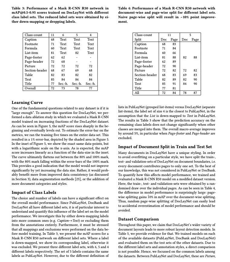
Document layout detection technology accurately identifies and locates elements such as titles, text blocks, and tables in a document, along with their spatial layout relationships. This serves as a core preliminary step in the intelligent document processing workflow, helping to build structured context for subsequent text analysis. In the context of rapid advancements in large language models, multimodal document understanding, and RAG (Retrieval-Augmented Generation) technology, high-quality structured data has become a crucial requirement for model training and knowledge base construction. With layout detection technology, we can automatically extract key information from document images, such as titles, authors, abstracts, keywords, publication years, journal names, and citation information, and combine it with OCR to recognize editable text. This information can be stored in a structured format, providing rich corpora for large model training data and offering strong support for the deep development of academic research.
First, you need to choose the corresponding PaddleX pipeline based on the task scenario. This section takes the post-processing optimization of layout detection results and regional text recognition with OCR as an example, aiming to obtain rich corpora information from document images. The corresponding PaddleX layout detection module can be used in the object detection pipeline. If you're unsure about the correspondence between tasks and pipelines, you can learn about the capabilities of related pipelines from the Model Pipeline List supported by PaddleX.
2. Supported Model List
- The layout detection model includes 23 common categories: document title, paragraph title, text, page number, abstract, table of contents, references, footnotes, header, footer, algorithm, formula, formula number, image, figure caption, table, table caption, seal, figure title, figure, header image, footer image, and sidebar text
| Model | Model Download Link | mAP(0.5) (%) | GPU Inference Time (ms) | CPU Inference Time (ms) | Model Storage Size (M) | Introduction |
|---|---|---|---|---|---|---|
| PP-DocLayout-L | Inference Model/Training Model | 90.4 | 34.5252 | 1454.27 | 123.76 M | A high-precision layout area localization model trained on a self-built dataset containing Chinese and English papers, magazines, contracts, books, exams, and research reports using RT-DETR-L. |
| PP-DocLayout-M | Inference Model/Training Model | 75.2 | 15.9 | 160.1 | 22.578 | A layout area localization model with balanced precision and efficiency, trained on a self-built dataset containing Chinese and English papers, magazines, contracts, books, exams, and research reports using PicoDet-L. |
| PP-DocLayout-S | Inference Model/Training Model | 70.9 | 13.8 | 46.7 | 4.834 | A high-efficiency layout area localization model trained on a self-built dataset containing Chinese and English papers, magazines, contracts, books, exams, and research reports using PicoDet-S. |
Note: The evaluation dataset for the above precision metrics is a self-built layout area detection dataset by PaddleOCR, containing 500 common document-type images of Chinese and English papers, magazines, contracts, books, exams, and research reports. GPU inference time is based on an NVIDIA Tesla T4 machine with FP32 precision. CPU inference speed is based on an Intel(R) Xeon(R) Gold 5117 CPU @ 2.00GHz with 8 threads and FP32 precision.
❗ The above list includes the 3 core models that are key supported by the text recognition module. The module actually supports a total of 11 full models, including several predefined models with different categories. The complete model list is as follows:
👉 Details of Model List
* Table Layout Detection Model| Model | Model Download Link | mAP(0.5) (%) | GPU Inference Time (ms) | CPU Inference Time (ms) | Model Storage Size (M) | Introduction |
|---|---|---|---|---|---|---|
| PicoDet_layout_1x_table | Inference Model/Training Model | 97.5 | 12.623 | 90.8934 | 7.4 M | A high-efficiency layout area localization model trained on a self-built dataset using PicoDet-1x, capable of detecting table regions. |
| Model | Model Download Link | mAP(0.5) (%) | GPU Inference Time (ms) | CPU Inference Time (ms) | Model Storage Size (M) | Introduction |
|---|---|---|---|---|---|---|
| PicoDet-S_layout_3cls | Inference Model/Training Model | 88.2 | 13.5 | 45.8 | 4.8 | A high-efficiency layout area localization model trained on a self-built dataset of Chinese and English papers, magazines, and research reports using PicoDet-S. |
| PicoDet-L_layout_3cls | Inference Model/Training Model | 89.0 | 15.7 | 159.8 | 22.6 | A balanced efficiency and precision layout area localization model trained on a self-built dataset of Chinese and English papers, magazines, and research reports using PicoDet-L. |
| RT-DETR-H_layout_3cls | Inference Model/Training Model | 95.8 | 114.6 | 3832.6 | 470.1 | A high-precision layout area localization model trained on a self-built dataset of Chinese and English papers, magazines, and research reports using RT-DETR-H. |
| Model | Model Download Link | mAP(0.5) (%) | GPU Inference Time (ms) | CPU Inference Time (ms) | Model Storage Size (M) | Introduction |
|---|---|---|---|---|---|---|
| PicoDet_layout_1x | Inference Model/Training Model | 97.8 | 13.0 | 91.3 | 7.4 | A high-efficiency English document layout area localization model trained on the PubLayNet dataset using PicoDet-1x. |
| Model | Model Download Link | mAP(0.5) (%) | GPU Inference Time (ms) | CPU Inference Time (ms) | Model Storage Size (M) | Introduction |
|---|---|---|---|---|---|---|
| PicoDet-S_layout_17cls | Inference Model/Training Model | 87.4 | 13.6 | 46.2 | 4.8 | A high-efficiency layout area localization model trained on a self-built dataset of Chinese and English papers, magazines, and research reports using PicoDet-S. |
| PicoDet-L_layout_17cls | Inference Model/Training Model | 89.0 | 17.2 | 160.2 | 22.6 | A balanced efficiency and precision layout area localization model trained on a self-built dataset of Chinese and English papers, magazines, and research reports using PicoDet-L. |
| RT-DETR-H_layout_17cls | Inference Model/Training Model | 98.3 | 115.1 | 3827.2 | 470.2 | A high-precision layout area localization model trained on a self-built dataset of Chinese and English papers, magazines, and research reports using RT-DETR-H. |
3. Quick Integration
❗ Before quick integration, please install the PaddleX wheel package. For detailed instructions, refer to PaddleX Local Installation Tutorial
First, obtain the default configuration file for the production line. Since the layout detection task is part of the object detection production line, you can execute the following command to obtain the default configuration file:
Save it in ./my_path/object_detection.yaml. By modifying the configuration file, you can customize various settings for the production line.
pipeline_name: object_detection

SubModules:
  ObjectDetection:
    module_name: object_detection
    model_name: PP-DocLayout-L  # Modify it to the layout region detection model name from the model list in the previous text.
    model_dir: null
    batch_size: 1
    img_size: null
    threshold: null
Subsequently, load the custom configuration file ./my_path/object_detection.yaml, and refer to the command-line method or Python script method in the local experience below for an online experience.
2.1 Local Experience — Command Line Method
Before running the following code, please download the sample image to your local machine. If the custom configuration file is saved in ./my_path/object_detection.yaml, you only need to execute:
paddlex --pipeline ./my_path/object_detection.yaml \
        --input layout_test_0.jpg \
        --threshold 0.5 \
        --save_path ./output/ \
        --device gpu:0
👉 After running, the result is: (Click to expand)
{'res': {'input_path': 'layout_test_0.jpg', 'page_index': None, 'boxes': [{'cls_id': 2, 'label': 'text', 'score': 0.9813319444656372, 'coordinate': [1194.3062, 1056.4965, 1435.4105, 1357.0413]}, {'cls_id': 2, 'label': 'text', 'score': 0.981147050857544, 'coordinate': [1194.2455, 725.1456, 1434.8359, 1049.3486]}, {'cls_id': 2, 'label': 'text', 'score': 0.9798598885536194, 'coordinate': [651.33997, 1243.4757, 892.80334, 1568.1959]}, {'cls_id': 1, 'label': 'image', 'score': 0.9786806106567383, 'coordinate': [654.7072, 535.5916, 1162.361, 871.6843]}, {'cls_id': 2, 'label': 'text', 'score': 0.9783889651298523, 'coordinate': [109.04134, 676.89685, 349.30542, 908.07996]}, {'cls_id': 2, 'label': 'text', 'score': 0.9776895046234131, 'coordinate': [922.3298, 1223.0814, 1164.6154, 1571.308]}, {'cls_id': 2, 'label': 'text', 'score': 0.9769193530082703, 'coordinate': [108.95575, 1778.8552, 350.25076, 2081.1873]}, {'cls_id': 2, 'label': 'text', 'score': 0.9768841862678528, 'coordinate': [1194.3513, 1363.4364, 1435.0712, 1568.2646]}, {'cls_id': 2, 'label': 'text', 'score': 0.9759471416473389, 'coordinate': [108.46416, 1517.3303, 349.46082, 1771.7134]}, {'cls_id': 2, 'label': 'text', 'score': 0.9742090106010437, 'coordinate': [651.50336, 1028.1143, 892.2849, 1236.0295]}, {'cls_id': 1, 'label': 'image', 'score': 0.9733730554580688, 'coordinate': [764.33875, 1602.9359, 1425.4358, 2066.0457]}, {'cls_id': 2, 'label': 'text', 'score': 0.9730471968650818, 'coordinate': [379.30127, 533.8668, 620.4098, 718.1861]}, {'cls_id': 2, 'label': 'text', 'score': 0.9729955196380615, 'coordinate': [446.23227, 1737.0651, 713.9191, 1896.8988]}, {'cls_id': 2, 'label': 'text', 'score': 0.9700003862380981, 'coordinate': [379.32547, 724.46204, 620.7275, 910.80316]}, {'cls_id': 2, 'label': 'text', 'score': 0.9692158699035645, 'coordinate': [379.22464, 1408.3339, 615.71564, 1567.7607]}, {'cls_id': 2, 'label': 'text', 'score': 0.968329668045044, 'coordinate': [108.44235, 1304.3308, 349.57904, 1511.2039]}, {'cls_id': 2, 'label': 'text', 'score': 0.9678011536598206, 'coordinate': [109.19986, 1017.0264, 349.31723, 1155.697]}, {'cls_id': 2, 'label': 'text', 'score': 0.9621286392211914, 'coordinate': [379.61563, 1262.9558, 620.6101, 1401.8175]}, {'cls_id': 2, 'label': 'text', 'score': 0.9615256190299988, 'coordinate': [379.74408, 1118.2937, 620.74426, 1256.6793]}, {'cls_id': 2, 'label': 'text', 'score': 0.958721935749054, 'coordinate': [1193.918, 532.8018, 1434.7432, 622.4289]}, {'cls_id': 2, 'label': 'text', 'score': 0.9559714198112488, 'coordinate': [922.562, 1080.9818, 1164.0387, 1215.7594]}, {'cls_id': 2, 'label': 'text', 'score': 0.9552412629127502, 'coordinate': [108.80721, 1161.9774, 349.6744, 1299.2362]}, {'cls_id': 2, 'label': 'text', 'score': 0.9507772922515869, 'coordinate': [109.40825, 580.92706, 349.14438, 670.02985]}, {'cls_id': 2, 'label': 'text', 'score': 0.949194073677063, 'coordinate': [1194.5726, 629.2398, 1434.1365, 718.40094]}, {'cls_id': 2, 'label': 'text', 'score': 0.9471532702445984, 'coordinate': [379.42627, 1021.85474, 619.82635, 1111.3379]}, {'cls_id': 2, 'label': 'text', 'score': 0.9420481324195862, 'coordinate': [652.1573, 930.8065, 887.3861, 1020.8891]}, {'cls_id': 2, 'label': 'text', 'score': 0.9257403016090393, 'coordinate': [922.33795, 932.40106, 1162.7422, 974.4318]}, {'cls_id': 0, 'label': 'paragraph_title', 'score': 0.8954867124557495, 'coordinate': [134.43443, 939.7384, 325.42734, 987.1273]}, {'cls_id': 0, 'label': 'paragraph_title', 'score': 0.8932625651359558, 'coordinate': [971.1828, 1004.2145, 1116.8691, 1052.5201]}, {'cls_id': 13, 'label': 'header', 'score': 0.8896792531013489, 'coordinate': [1129.3605, 160.20511, 1260.6161, 193.23979]}, {'cls_id': 0, 'label': 'paragraph_title', 'score': 0.8894897699356079, 'coordinate': [404.63666, 944.63464, 597.64923, 992.9647]}, {'cls_id': 13, 'label': 'header', 'score': 0.8644265532493591, 'coordinate': [411.9833, 174.19376, 922.93945, 194.1207]}, {'cls_id': 3, 'label': 'number', 'score': 0.7865270376205444, 'coordinate': [1385.2574, 155.55762, 1418.2019, 194.63576]}, {'cls_id': 0, 'label': 'paragraph_title', 'score': 0.7727568745613098, 'coordinate': [485.61816, 1676.4192, 676.21356, 1699.8445]}, {'cls_id': 2, 'label': 'text', 'score': 0.7702363729476929, 'coordinate': [642.1937, 1925.9141, 714.12067, 1945.3125]}, {'cls_id': 11, 'label': 'doc_title', 'score': 0.7163856625556946, 'coordinate': [127.23631, 301.37003, 1316.9393, 473.41168]}, {'cls_id': 6, 'label': 'figure_title', 'score': 0.6773825287818909, 'coordinate': [657.4694, 892.38696, 1162.7767, 910.70337]}, {'cls_id': 2, 'label': 'text', 'score': 0.6245782375335693, 'coordinate': [110.19977, 534.36707, 318.00195, 554.423]}, {'cls_id': 13, 'label': 'header', 'score': 0.5930579304695129, 'coordinate': [130.28291, 144.46971, 308.31525, 197.32173]}, {'cls_id': 20, 'label': 'header_image', 'score': 0.5242483019828796, 'coordinate': [130.28291, 144.46971, 308.31525, 197.32173]}]}}
[xmin, ymin, xmax, ymax].
The visualized image is as follows:

2.2 2.2 Local Experience — Python Method
The above command-line method allows you to quickly experience and check the results. In projects, code integration is often required. You can achieve quick inference in production with the following lines of code:
from paddlex import create_pipeline

pipeline = create_pipeline(pipeline="./my_path/object_detection.yaml")

output = pipeline.predict("layout_test_0.jpg", threshold=0.5)
for res in output:
    res.print()
    res.save_to_img("./output/")
    res.save_to_json("./output/")
The output printed by the code will be consistent with the results from the command-line experience mentioned earlier.
4. Production Post-processing Optimization.
The production pipeline for layout detection models offers various post-processing optimization techniques to help you further improve prediction results. For the post-processing parameters that can be passed into the predict method, please refer to the Layout Area Detection Usage Tutorial. Below, we will introduce how to use these optimization techniques based on the layout detection model production pipeline.
4.1 Dynamic Threshold Optimization — Can Optimize Missed and False Detections
The layout detection model supports dynamic threshold adjustment. You can pass the threshold parameter, which supports either a float or a dictionary of custom thresholds for each category, allowing you to set a specific detection score threshold for each category. This means you can flexibly adjust for missed or false detections based on your own data, ensuring more accurate detections each time. The category-to-ID mapping for the PP-DocLayout series models is as follows:
{'paragraph_title': 0, 'image': 1, 'text': 2, 'number': 3, 'abstract': 4, 'content': 5,
'figure_title': 6, 'formula': 7, 'table': 8, 'table_title': 9, 'reference': 10, 'doc_title': 11, 'footnote': 12, 'header': 13, 'algorithm': 14, 'footer': 15, 'seal': 16, 'chart_title': 17, 'chart': 18, 'formula_number': 19, 'header_image': 20, 'footer_image': 21, 'aside_text': 22}
Before running the following code, please download the sample image to your local machine.
from paddlex import create_pipeline

pipeline = create_pipeline(pipeline="./my_path/object_detection.yaml") # 阈值参数不设置时,默认为0.5
output = pipeline.predict("layout_test_2.jpg")
for res in output:
    res.print()
    res.save_to_img("./output/")
    res.save_to_json("./output/")
You may notice that in the image on the left, there is an incorrect text category box identified in the upper right corner.
In this case, you can enable threshold={2: 0.6} to set the detection score threshold to 0.6 specifically for the text category, whose category ID is 2. This adjustment can filter out the incorrect text box, while the default threshold of 0.5 is retained for other categories. Execute the following code:
from paddlex import create_pipeline

pipeline = create_pipeline(pipeline="./my_path/object_detection.yaml")
output = pipeline.predict("layout_test_2.jpg", threshold={2: 0.6}) # To set the detection score threshold specifically for category 2 (text) to 0.6 while keeping the default threshold of 0.5 for other categories
for res in output:
    res.print()
    res.save_to_img("./output/")
    res.save_to_json("./output/")
In the save directory, you can view the visualization results as follows. You will notice that the extra box in the upper right corner of the image below has been filtered out by the threshold, leaving only the optimal detection results:

0.5

threshold={2: 0.6}
4.2 Overlapping Box Filtering — Eliminating Redundant Box Interference
The layout_nms parameter is used for overlapping box filtering. It is a boolean type used to specify whether to use NMS (Non-Maximum Suppression) to filter overlapping boxes. Enabling this feature allows for the automatic selection of the optimal detection results and eliminates redundant interfering boxes. By default, the overlapping box filtering feature is turned off. To enable this feature, you need to pass the parameter layout_nms=True in the predict method. Execute the following code with layout_nms=False to disable the overlapping box filtering feature and view the results.
When the overlapping box filtering feature is not enabled, you may notice overlapping box interference in the upper right corner of the image on the left. In this case, you can enable layout_nms=True to filter out the redundant boxes and see that the extra box in the upper right corner of the image on the right has been filtered out, leaving only the optimal detection results. Execute the code for both disabling and enabling the filtering feature to view and compare the results:
from paddlex import create_pipeline

pipeline = create_pipeline(pipeline="./my_path/object_detection.yaml")
# output = pipeline.predict("layout_test_2.jpg", threshold=0.5)  # Disabling the overlapping box filtering feature
output = pipeline.predict("layout_test_2.jpg", threshold=0.5, layout_nms=True)  # Enabling the overlapping box filtering feature
for res in output:
    res.print()
    res.save_to_img("./output/")
    res.save_to_json("./output/")
The visual comparison of the results is as follows:
not setting

layout_nms=True
4.3 Adjustable Box Side Length — Obtaining Complete Blocks
The layout_unclip_ratio parameter allows you to adjust the side length of the box, no longer restricted to a fixed box size. By adjusting the scaling factor of the detection box, you can freely expand or contract the side length of the box while keeping the center point unchanged. This helps in outputting the correct and complete content of the layout area.
from paddlex import create_pipeline

pipeline = create_pipeline(pipeline="./my_path/object_detection.yaml")
# output = pipeline.predict("layout_test_2.jpg",  threshold={2: 0.6})  # Without adjusting the scaling factor of the detection box
output = pipeline.predict("layout_test_2.jpg",  threshold={2: 0.6}, layout_unclip_ratio=(1.0, 1.05))  # Adjust the scaling factor of the height of the detection box to 1.05.
for res in output:
    res.print()
    res.save_to_img("./output/")
    res.save_to_json("./output/")
The visualization results in the saved directory are as follows. It can be observed that by adjusting the scaling factor of the detection box to layout_unclip_ratio=(1.0, 1.05), a taller area can be obtained.
not setting

(1.0, 1.05)
4.4 Box Merging Mode — Focusing on the Whole or Details
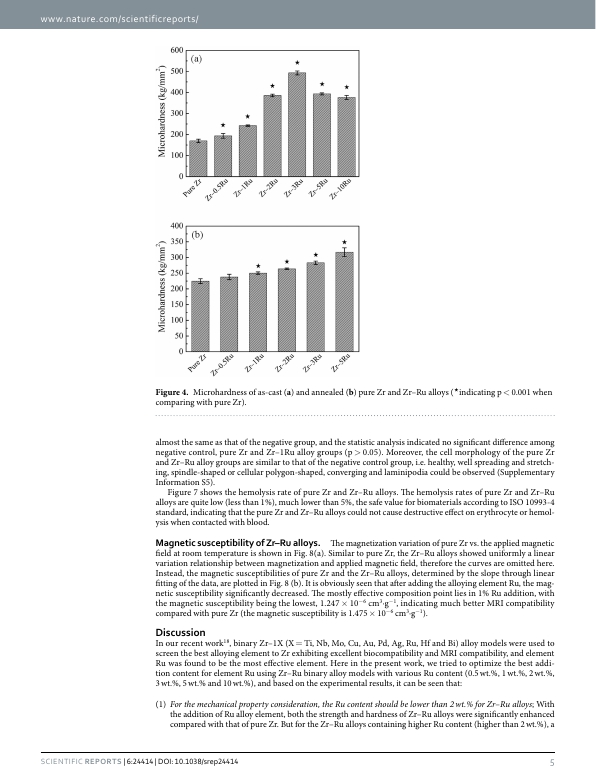
layout_merge_bboxes_mode: This parameter defines the box merging mode for the detection boxes output by the model. You can choose "large" to retain the outer box or "small" to retain the inner box, with the default setting retaining all boxes if not specified. For example, if there are multiple subplots within a chart area, selecting the "large" mode will retain one large box for the entire chart, facilitating an overall understanding of the chart area and restoring its position on the layout. On the other hand, selecting "small" will retain multiple boxes for each subplot, allowing for individual understanding or processing of each subplot. Execute the code below to experience the differences in results when the layout_merge_bboxes_mode parameter is not set, set to 'large', and set to 'small'. Execute the code below to view the results. Download the sample image to your local machine.
from paddlex import create_pipeline

pipeline = create_pipeline(pipeline="./my_path/object_detection.yaml")
output = pipeline.predict("PMC4836298_00004.jpg") # not setting
# output = pipeline.predict("PMC4836298_00004.jpg", layout_merge_bboxes_mode="small") # 'small' mode
# output = pipeline.predict("PMC4836298_00004.jpg", layout_merge_bboxes_mode="large") # 'large' mode
for res in output:
    res.print()
    res.save_to_img("./output/")
    res.save_to_json("./output/")
In the saved directory, the comparison of visualization results is as follows. By observing the prediction differences for the chart category, you can see that when the layout_merge_bboxes_mode parameter is not set, all boxes are retained. When set to the "large" mode, the boxes are merged into one large chart box, which facilitates an overall understanding of the chart area and the restoration of the chart's position on the layout. When set to the "small" mode, multiple boxes for each subplot are retained, allowing for individual understanding or processing of each subplot.
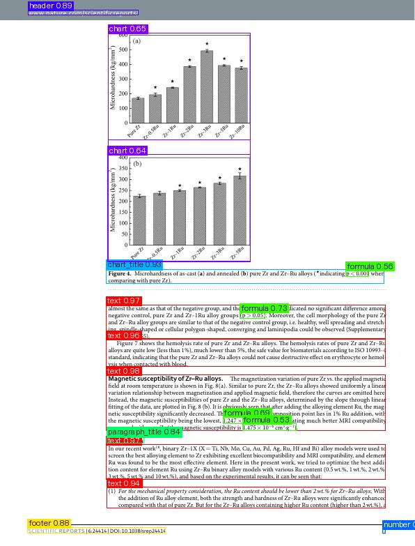
not setting

large mode

small mode
5. Layout Detection and OCR Combination
PaddleX offers a wide variety of models and model pipelines tailored for different tasks. Additionally, PaddleX supports the combination of multiple models to tackle complex and specific tasks. On top of the layout area detection pipeline, you can further integrate OCR recognition components to extract text content from layout areas. This provides corpus data for subsequent tasks such as large model text content understanding and summary generation. Before running the code below, please download the sample image to your local machine. Execute the following code to view the results.
import cv2
from paddlex import create_pipeline

class LayoutOCRPipeline():

    def __init__(self):
        self.layout_pipeline = create_pipeline(pipeline="./my_path/object_detection.yaml")  # Load the custom configuration file mentioned above to create a layout detection pipeline.
        self.ocr_pipeline = create_pipeline(pipeline="OCR") # init OCR pipeline

    def crop_table(self, layout_res, layout_name):
        img_path = layout_res["input_path"]
        img = cv2.imread(img_path)
        table_img_list = []
        for box in layout_res["boxes"]:
            if box["label"] != layout_name: # only obtain layout_name box
                continue
            xmin, ymin, xmax, ymax = [int(i) for i in box["coordinate"]]
            table_img = img[ymin:ymax, xmin:xmax]
            table_img_list.append(table_img)
        return table_img_list

    def predict(self, data, layout_name):
        for layout_res in self.layout_pipeline.predict(data):  # do layout detection
            final_res = {}
            crop_img_list = self.crop_table(layout_res, layout_name) # crop box
            if len(crop_img_list) == 0:
                continue
            ocr_res = list(self.ocr_pipeline.predict(    # do OCR
                                                input=crop_img_list,
                                                use_doc_orientation_classify=False,
                                                use_doc_unwarping=False,
                                                use_textline_orientation=False
                                                ))
            final_res[layout_name] = [res["rec_texts"] for res in ocr_res]
            yield final_res


if __name__ == "__main__":
    solution = LayoutOCRPipeline()
    output = solution.predict("layout_test_0.jpg", layout_name="paragraph_title") # focus only on the areas containing paragraph titles
    for res in output:
        print(res)
The output is as follows:
{'paragraph_title': [['柔性执法', '好事办在群众心坎上'], ['缓解“停车难”', '加强精细化治理'], ['“潮汐”摊位', '聚拢文旅城市烟火气'], ['普法宣传“零距离”']]}
It is evident that the text content of paragraph titles has been correctly extracted, forming structured data that can be provided as training data for large models to be used in tasks such as text content understanding and summary generation.
Note: This section mainly demonstrates how to combine layout detection and OCR recognition. In practice, PaddleX has already provided a variety of feature-rich pipelines. You can refer to the PaddleX Pipeline List for more information.
6. Development Integration/Deployment
If the layout detection performance meets your requirements for inference speed and accuracy in production, you can proceed directly with development integration/deployment.
6.1 Directly apply the adjusted post-processing pipeline in your Python project. You can refer to the following sample code:
from paddlex import create_pipeline

pipeline = create_pipeline(pipeline="./my_path/object_detection.yaml")
output = pipeline.predict("layout_test_2.jpg", threshold=0.5, layout_nms=True, layout_merge_bboxes_mode="large")
for res in output:
    res.print()
    res.save_to_img("./output/")
    res.save_to_json("./output/")
6.2 Deploying with High Stability as a Service is the practical content of this tutorial. You can refer to the PaddleX Service Deployment Guide for implementation.
Please note that the current high-stability service deployment solution only supports the Linux operating system.
6.2.1 Obtaining the SDK
Download the Object Detection High Stability Service Deployment SDK from paddlex_hps_object_detection_sdk.tar.gz, extract the SDK, and run the deployment script as follows:
6.2.2 Obtaining the Serial Number
- In the "Open Source Model Pipeline Deployment Serial Number Consultation and Acquisition" section of the PaddlePaddle AI Studio Galaxy Community - AI Learning and Training Community, select "Get Now," as shown in the image below:
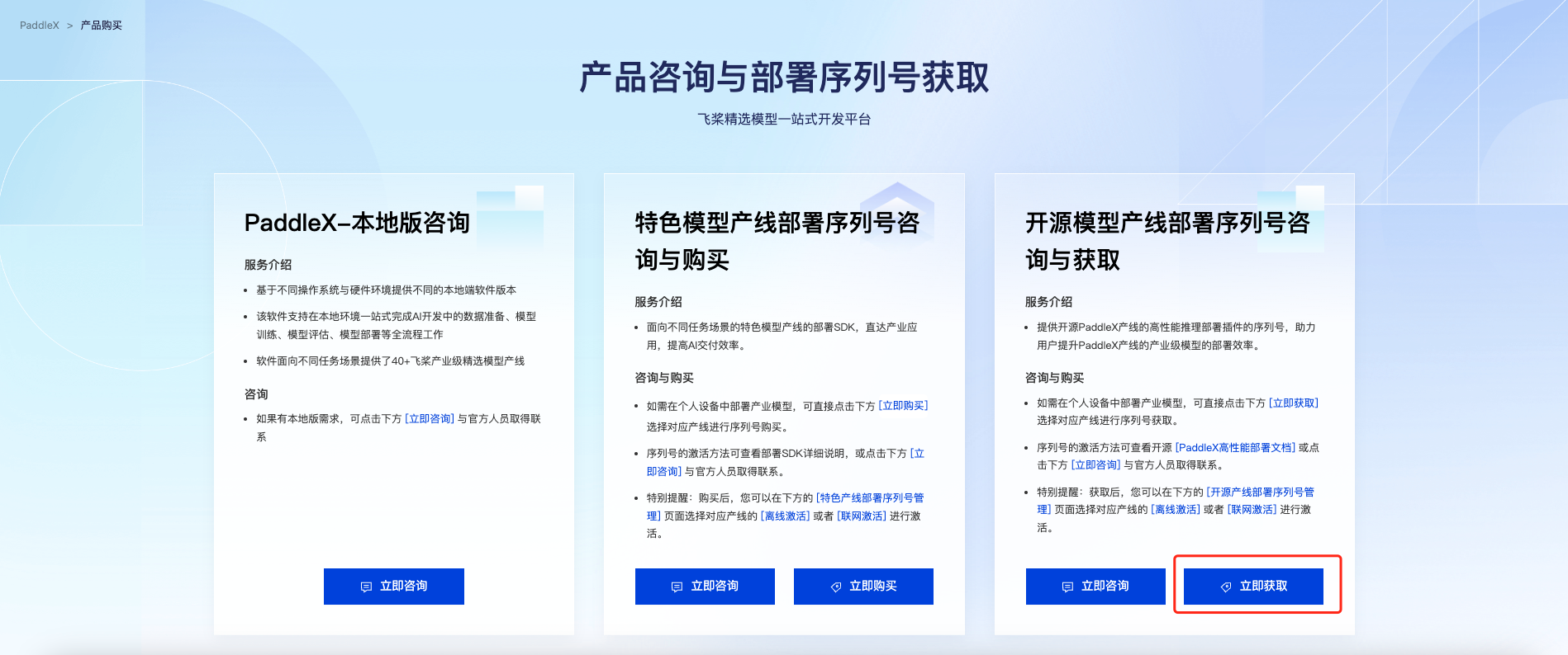
Select the target detection pipeline and click "Get." Then, you can find the acquired serial number in the "Open Source Pipeline Deployment SDK Serial Number Management" section at the bottom of the page:
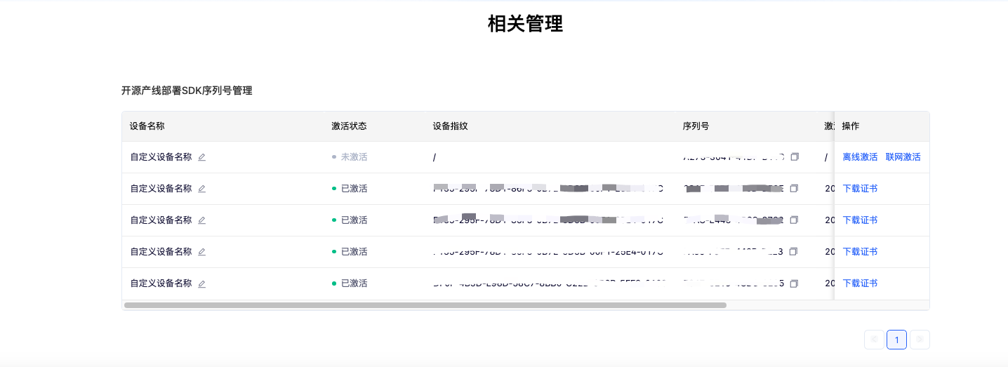
Please Note: Each serial number can only be bound to a unique device fingerprint and can only be bound once. This means that if you are deploying pipelines using different machines, you must prepare a separate serial number for each machine.
6.2.3 Running the Service
To run the service:
-
For images that support deployment using NVIDIA GPUs (the machine needs to have an NVIDIA driver installed that supports CUDA 11.8):
-
For CPU-only images:
Once the image is ready, switch to the server directory and execute the following command to run the server:
docker run \
    -it \
    -e PADDLEX_HPS_DEVICE_TYPE={deployment device type} \
    -e PADDLEX_HPS_SERIAL_NUMBER={LICENSE} \
    -e PADDLEX_HPS_UPDATE_LICENSE=1 \
    -v "$(pwd)":/workspace \
    -v "${HOME}/.baidu/paddlex/licenses":/root/.baidu/paddlex/licenses \
    -v /dev/disk/by-uuid:/dev/disk/by-uuid \
    -w /workspace \
    --rm \
    --gpus all \
    --init \
    --network host \
    --shm-size 8g \
    {docker name} \
    /bin/bash server.sh
- The deployment device type can be either
cpuorgpu. The CPU-only image only supportscpu. - If you wish to deploy using the CPU, you do not need to specify
--gpus. -
The above commands can only be executed successfully after activation. PaddleX provides two activation methods: offline activation and online activation. The details are as follows:
- Online Activation: Set
PADDLEX_HPS_UPDATE_LICENSEto1during the first execution to allow the program to automatically update the certificate and complete activation. For subsequent executions, you can setPADDLEX_HPS_UPDATE_LICENSEto0to avoid updating the certificate online. - Offline Activation: Follow the instructions in the serial number management section to obtain the machine's device fingerprint and bind the serial number with the device fingerprint to obtain the certificate and complete activation. For this activation method, you need to manually place the certificate in the
${HOME}/.baidu/paddlex/licensesdirectory on the machine (create the directory if it does not exist). When using this method, setPADDLEX_HPS_UPDATE_LICENSEto0to avoid updating the certificate online.
- Online Activation: Set
-
Ensure that
/dev/disk/by-uuidon the host machine exists and is not empty, and that the directory is mounted correctly to execute the activation successfully. - If you need to enter the container for debugging, you can replace
/bin/bash server.shin the command with/bin/bash, and then execute/bin/bash server.shinside the container. - If you want the server to run in the background, you can replace
-itwith-din the command. After the container starts, you can view the container logs usingdocker logs -f {container ID}. - Add
-e PADDLEX_USE_HPIP=1in the command to use the PaddleX High-Performance Inference Plugin to accelerate the inference process. However, please note that not all pipelines support the use of the high-performance inference plugin. Please refer to the PaddleX High-Performance Inference Guide for more information.
You may observe output similar to the following:
I1216 11:37:21.601943 35 grpc_server.cc:4117] Started GRPCInferenceService at 0.0.0.0:8001
I1216 11:37:21.602333 35 http_server.cc:2815] Started HTTPService at 0.0.0.0:8000
I1216 11:37:21.643494 35 http_server.cc:167] Started Metrics Service at 0.0.0.0:8002
6.2.4 To call the service
Currently, only the Python client is supported for calling the service. The supported Python versions are 3.8 to 3.12.
Switch to the client directory of the high-stability service deployment SDK and run the following command to install the dependencies:
# 建议在虚拟环境中安装
python -m pip install -r requirements.txt
python -m pip install paddlex_hps_client-*.whl
The client.py script in the client directory contains examples of service calls and provides a command-line interface.
6.3 In addition, PaddleX offers three other deployment methods, as described below:
- high-performance inference: In actual production environments, many applications have stringent standards for deployment strategy performance metrics (especially response speed) to ensure efficient system operation and smooth user experience. To this end, PaddleX provides high-performance inference plugins aimed at deeply optimizing model inference and pre/post-processing for significant end-to-end process acceleration. For detailed high-performance inference procedures, please refer to the PaddleX High-Performance Inference Guide.
- Service-Oriented Deployment: Service-oriented deployment is a common deployment form in actual production environments. By encapsulating inference functions as services, clients can access these services through network requests to obtain inference results. PaddleX supports users in achieving cost-effective service-oriented deployment of production lines. For detailed service-oriented deployment procedures, please refer to the PaddleX Service-Oriented Deployment Guide.
- Edge Deployment: Edge deployment is a method that places computing and data processing capabilities directly on user devices, allowing devices to process data without relying on remote servers. PaddleX supports deploying models on edge devices such as Android. For detailed edge deployment procedures, please refer to the PaddleX Edge Deployment Guide.
You can choose the appropriate method to deploy the model pipeline based on your needs, and then proceed with the subsequent integration of AI applications.